RANS Channel
This tutorial describes the essential setup details for a wall-resolved RANS simulation, illustrated through a turbulent channel flow case. The \(k-\tau\) and \(k-\tau SST\) RANS models are employed for this tutorial. More information on the \(k-\tau\) model can be found here.
Before You Begin
It is highly recommended that new users familiarize themselves with the basic NekRS simulation setup files and procedures outlined in the Fully Developed Laminar Flow tutorial.
Mesh and Boundary Conditions
The mesh is generated with genbox utility using the following input file
-3                     spatial dimension  (will create box.re2)
3                      number of fields
#=======================================================================
#
Box
-5  -12  -3                     nelx,nely,nelz for Box
0 8 1.                          x0,x1,gain  (rescaled in usrdat)
-1 0 1.                          y0,y1,gain  (rescaled in usrdat)
0 1 1.                          z0,z1,gain
P  ,P  ,W  ,SYM,P  ,P           Velocity BCs
P  ,P  ,t  ,I  ,P  ,P           k-equation BCs
P  ,P  ,t  ,I  ,P  ,P           tau-equation BCs
It creates an infinite 3D half-channel of non-dimensional width \(1\).
The streamwise (\(x\)) direction has 5 elements with periodic (P) boundary conditions.
The wall-normal (\(y\)) direction has 12 elements with a symmetry (SYM) boundary condition specified at the top face and a wall (W) boundary on the bottom face.
Corresponding boundary conditions for the \(k\) and \(\tau\) transport equations are insulated (I) at the symmetry boundary and Dirichlet (t) type (equal to zero) at the wall.
The spanwise (\(z\)) direction has 3 elements with periodic (P) boundary conditions.
The mesh is further modified in the .udf file to refine it near the wall to resolve boundary layers, as explained in following sections.
Control Parameters (.par file)
Details of the structure of the parameter file can be found here. The parameter file for this case is as follows,
userSections = CASEDATA

[GENERAL]
polynomialOrder = 5

stopAt = endTime
endTime = 1100
dt = 5e-02
timeStepper = tombo2

checkpointControl = simulationTime
checkpointInterval = 100

constFlowRate = meanVelocity=1.0 + direction=X

scalars = k, tau

[PROBLEMTYPE]
equation = navierStokes+variableViscosity

[FLUID PRESSURE]
residualTol = 1e-04

[FLUID VELOCITY]
residualTol = 1e-06
rho = 1.0
viscosity = 1/43500.

[SCALAR TAU]
residualTol = 1e-08

[SCALAR K]
residualTol = 1e-08

[CASEDATA]
MODEL = KTAU
#MODEL = KTAUSST
For RANS simulations it is critical to include two additional scalars which correspond to the \(k\) and \(\tau\) fields respectively.
This is done using the scalars key in [GENERAL] section by the string identifiers "k" and "tau" as shown above.
In addition, it is essential to also include the [PROBLEMTYPE] card and specify the equation key as navierStokes+variableViscosity.
This ensures that a spatially varying diffusion field can be used to include eddy viscosity in the RANS momentum equation, as discussed here.
For this particular tutorial, the simulation is non-dimensionalized and flow properties are rho=1.0 and viscosity=1/43500.
The properties are assigned in .par file under the [FLUID VELOCITY] section as shown above.
[SCALAR K] and [SCALAR TAU] sections must also be included in the .par file.
Warning
For RANS cases, no transport properties must be assigned under the [SCALAR K] and [SCALAR TAU] sections.
These are assigned internally by NekRS.
If any properties are assigned under these sections, the solver with throw an informative error and exit.
It is strongly recommended to run RANS simulations in non-dimensional form.
This setup corresponds to \(Re = 43,500\), which is well above the critical Reynolds number for a channel.
The specified non-dimensional bulk velocity for the case is \(U_b=1\).
NekRS offers an inbuilt mechanism to maintain and control a specified control rate in periodic domains.
This is assigned through the constFlowRate key in [GENERAL] section, as shown above.
The key takes two parameters, viz., meanVelocity which is assigned the value of bulk velocity and direction takes the direction of streamwise velocity component.
The case corresponds to one of the DNS simulation performed by Lee and Moser [Lee2015] for turbulent channel flow.
Further, in this example a user section is included to specify the RANS model through the .par file in CASEDATA.
Note that two models are included in the example, KTAU and KTAUSST.
The user can conveniently choose either model by assigning the value to MODEL key, as shown above.
This is parsed in the .udf as explained in following section.
User-defined Host Functions File (.udf file)
All RANS models in NekRS are available as plugins. Generic details on RANS setup can be found in the setup guide here.
To get started, include the RANS header at the top of the .udf file,
#include "RANSktau.hpp"
The required internal arrays and data structures for RANS models are initialized in the UDF_Setup routine.
For this case the UDF_Setup setup is as follows,
}

void UDF_Setup()
{
  nrs->userProperties = &uservp;
  nrs->userSource = &userq;

  auto mesh = nrs->meshV;

  // Box mesh manipulation
  const auto beta = 2.8;
  auto [x, y, z] = mesh->xyzHost();

  for (int n = 0; n < mesh->Nlocal; n++) {
    y[n] = tanh(beta * y[n]) / tanh(beta);
  }
  mesh->o_y.copyFrom(y.data());

  //Initial Conditions
  std::vector<dfloat> U(mesh->dim * nrs->fluid->fieldOffset, 0.0);
  std::vector<dfloat> k(mesh->Nlocal, 0.0);
  std::vector<dfloat> tau(mesh->Nlocal, 0.0);

  if (platform->options.getArgs("RESTART FILE NAME").empty()) {
    auto& scalar = nrs->scalar;
    for(int n = 0; n < mesh->Nlocal; n++) {
      U[n + 0 * nrs->fluid->fieldOffset] = 1;
      U[n + 1 * nrs->fluid->fieldOffset] = 0;
      U[n + 2 * nrs->fluid->fieldOffset] = 0;
      k[n] = 0.01;
      tau[n] = 0.1;
    }
    nrs->fluid->o_U.copyFrom(U.data(), U.size());
    nrs->scalar->o_solution("k").copyFrom(k.data(), k.size());
    nrs->scalar->o_solution("tau").copyFrom(tau.data(), tau.size());
  }

  std::string model = "ktau";
  platform->par->extract("casedata","model",model);
Several operations are performed in the code snippet above.
Diffusion and Source terms
nrs->userProperties and nrs->userSource are internal pointer variables which must be assigned user defined routines for specifying spatially varying transport properties and source terms, respectively.
uservp and userq are the corresponding routines which must be specified in .udf file, as shown below,
}

void uservp(double time)
{
  RANSktau::updateProperties();
}

void userq(double time)
{
NekRS provides convenient routines, available in the namespace RANSktau, for spatially varying diffusion and source terms, as shown above.
Details on the diffusion and source terms can be found in RANS theory.
Mesh Modification
Further, the UDF_Setup routine contains code to modify mesh y-coordinates for this case, in order to have fine boundary layers near the wall.
mesh->xyzHost() call is used to fetch the pointers to the existing x, y and z coordinate arrays on the host.
Note that these variables are std::vector`, dynamic container arrays.
Subsequently, the for loop goes through all GLL points in the mesh and modifies the y-coordinate, based on a hyperbolic tangent profile.
After modifying the coordinates on the host, the arrays must also be copied to the device arrays, mesh->o_y, using the copyFrom call.
Initial Conditions
Next essential operation that must be included in .udf file is initialization of velocity, \(k\) and \(\tau\) fields.
In this example, the x-component of velocity is initialized to a uniform value of 1, \(k\) to 0.01 and \(\tau\) to 0.1.
Note
The \(k\) and \(\tau\) fields can be initialized to any reasonable positive value. For non-dimensional runs, 0.01 and 0.1 can be used as initial values. It is not recommended to initial these fields to zero, to avoid division by zero of some source terms.
RANS Setup
The final essential operation that must be included in UDF_Setup is the call to RANSktau::setup routine.
This function requires one essential parameter, which is the index of the \(k\) scalar field, nrs->scalar->nameToIndex.find("k")->second.
The second parameter is optional and specifies the RANS model name.
If a second parameter is not passed, NekRS defaults to the standard \(k-\tau\) RANS model.
Note that for this case the model type is specified in .par file in [CASEDATA] section and read in UDF_Setup by extracting using the platform->par->extract function, as shown.
See the RANS guide for all RANS models available in NekRS and how to specify them.
Boundary Conditions
The boundary conditions for \(k\) and \(\tau\) scalar fields on the channel wall are specified in the OKL block in the udfDirichlet device function as follows,
#ifdef __okl__

void udfDirichlet(bcData *bc)
{
  if(isField("scalar k") || isField("scalar tau")) {
    bc->sScalar = 0;
  }
}
isField() function helps identify the scalar field using the string identifier specified in .par file.
Note that the boundary condition on the wall for both \(k\) and \(\tau\) transport equations are zero.
Execute Step Routine
The final essential routine in .udf is the UDF_ExecuteStep routine:
void UDF_ExecuteStep(double time, int tstep)
{
  //if (nrs->lastStep) {
  //  computeUtau(nrs, time, tstep);
  //  extractLine(nrs, time);
  //}
}
Any case specific post-processing can be performed in this routine.
nrs->lastStep identifies the last step in the simulation and it can be used to perform any post-processing operations before the simulation terminates.
For this case, two optional post-processing routines are provided, explained in the following sections.
Compilation and Running
All required case files for RANS wall-resolved channel simulation can be downloaded using the links below:
If for some reason you encountered an insurmountable error and were unable to generate any of the required files, you may use the provided links to download them. Now you can run the case.
$ nrsbmpi channel 4
The above command will launch an MPI jobs on your local machine using 4 ranks.
The output will be redirected to logfile.
Results
For reference, the results obtained from the \(k-\tau\) and \(k-\tau SST\) RANS wall-resolved models are shown below:
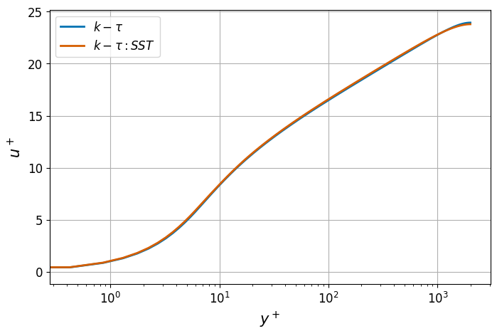
Fig. 11 Normalized stream-wise velocity from different RANS models.
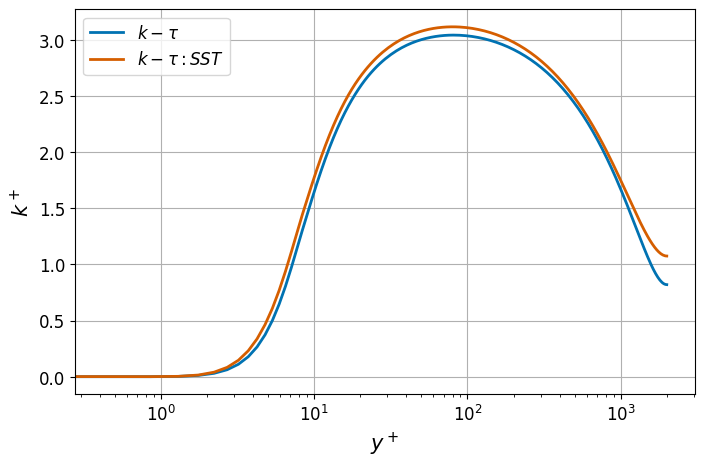
Fig. 12 Normalized TKE from different RANS models.
Optional: Post-processing Routines
For the convenience of the user, post-processing routines are provided in the above downloadable .udf file.
The routines are specific to this case, but may be adopted for other cases with suitable modifications.
Data Extraction Along a Line
The routine shown below extracts x-component of velocity and \(k\) profile along 200 data points distributed along a vertical line from \((7,-1,0.5)\) to \((7,0,0.5)\).
NekRS offers inbuilt interpolation routines to find the value of any field at a specified point in the domain.
interpolator->eval call evaluates the value of velocity and \(k\) at the points stored in arrays xp, yp, zp.
The extracted data is written into a file named profile.dat.
More details on the usage of interpolation routines can be found here.
void extractLine(nrs_t *nrs, double time)
{
  const auto np = (platform->comm.mpiRank() == 0) ? 200 : 0;
  const auto offset = np;

  static pointInterpolation_t *interpolator = nullptr;
  static std::vector<dfloat> xp, yp, zp;
  static deviceMemory<dfloat> o_Up;
  static deviceMemory<dfloat> o_kp;

  if (!interpolator) {
    auto mesh = nrs->meshV;
    const auto yMin = platform->linAlg->min(mesh->Nlocal, mesh->o_y, platform->comm.mpiComm());
    const auto yMax = platform->linAlg->max(mesh->Nlocal, mesh->o_y, platform->comm.mpiComm());

    if (np) {
      const auto x0 = 7.0;
      const auto z0 = 0.5;

      xp.push_back(x0);
      yp.push_back(yMin);
      zp.push_back(z0);

      const auto betaY = 2.8;
      const auto dy = (yMax - yMin) / (np - 1);
      for (int i = 1; i < np - 1; i++) {
        xp.push_back(x0);
        yp.push_back(tanh(betaY * (i * dy - 1)) / tanh(betaY));
        zp.push_back(z0);
      }

      xp.push_back(x0);
      yp.push_back(yMax);
      zp.push_back(z0);
      o_Up.resize(offset);
      o_kp.resize(offset);
    }

    interpolator = new pointInterpolation_t(mesh, platform->comm.mpiComm());
    interpolator->setPoints(xp, yp, zp);
    interpolator->find();
  }

  interpolator->eval(1, nrs->fluid->fieldOffset, nrs->fluid->o_U, offset, o_Up);
  interpolator->eval(1, nrs->fluid->fieldOffset, nrs->scalar->o_solution("k"), offset, o_kp);

  if (platform->comm.mpiRank() == 0) {
    std::vector<dfloat> Up(np);
    std::vector<dfloat> kp(np);
    o_Up.copyTo(Up);
    o_kp.copyTo(kp);

    std::ofstream f("profile.dat");
    for (int i = 0; i < np; i++) {
      f << std::scientific << time << " " << yp[i] << " " << Up[i] << " " << kp[i] << std::endl;
    }
    f.close();
  }
}
Compute Friction Velocity
The following routine computes the surface averaged friction velocity evaluated at all walls in the domain. The local friction velocity at any boundary GLL point is defined as,
where \(\vec{n}\) is the local normal vector at the boundary. The average friction velocity is computed as,
where \(\Gamma\) represents all wall boundaries. The routine is as follows. It also computes the relative error in computed mean friction velocity compared to the DNS value reported by [Lee2015]. For further details on the NekRS routine used below, see Postprocessing.
void computeUtau(nrs_t *nrs, double time, int tstep)
{
  auto mesh = nrs->meshV;

  std::vector<int> wbID;
  for (auto &[key, bcID] : platform->app->bc->bIdToTypeId()) {
    const auto field = key.first;
    if (field == "fluid velocity") {
      if (bcID == bdryBase::bcType_zeroDirichlet) {
        wbID.push_back(key.second + 1);
      }
    }
  }
  auto o_wbID = platform->device.malloc<int>(wbID.size(), wbID.data());

  auto o_Sij = nrs->strainRate();

  auto forces = nrs->aeroForces(o_wbID, o_Sij);
  o_Sij.free();

  auto o_tmp = platform->deviceMemoryPool.reserve<dfloat>(mesh->Nlocal);
  platform->linAlg->fill(mesh->Nlocal, 1.0, o_tmp);
  const auto areaWall = mesh->surfaceAreaMultiplyIntegrate(o_wbID, o_tmp);

  // https://turbulence.oden.utexas.edu/channel2015/data/LM_Channel_2000_mean_prof.dat
  const auto utauRef = 4.58794e-02;
  const auto utau = sqrt(std::abs(forces->tangential()[0]) / areaWall);
  const auto utauErr = std::abs((utau - utauRef) / utauRef);
  if (platform->comm.mpiRank() == 0)
    printf("utau: %.4e; utauErr: %.4e \n", utau, utauErr);
}