Mesh & Meshing

This chapter describes how to configure mesh-related options in NekRS and outlines common workflows for generating, importing, and modifying meshes. For practical guidance on mesh quality and refinement strategies, see Meshing Tips.

A quick overview:

• Runtime Setup to load and modify meshes, boundary tags and connectivity

• Generate simple meshes with Nek5000 Meshing Tools

• Convert External Meshes from Gmsh, Exodus II, and CGNS

Related topics:

• Moving Mesh setup

• Conjugate Heat Transfer meshes

• On-the-fly h-Refinement

• Additional meshing tips

• Overview of mesh_t

Runtime Setup

Meshes are stored in the binary re2 file, which contains the coordinates and boundary tags. Several aspects of the mesh can still be adjusted at runtime in a flexible way.

Coordinates Modification

Like Nek5000, NekRS allows mesh coordinates to be modified at runtime. Static, one-time deformations are typically applied during initialization in usrdat2 in the usr file or UDF_Setup() in the .udf file.

In principle, any mesh point can be moved arbitrarily, as long as the mapping remains valid—non-self-intersecting with a positive Jacobian. Below we show examples of common operations implemented in usrdat2 (in the .usr file), including uniform scaling for non-dimensionalization, rotations, and wall-normal stretching.

Uniform scaling (pb146)Domain rescaling (tgv)Rotation (shlChannel)Wall-normal stretching (ktauChannel)

In the pb146 example, the mesh is rescaled so that the radius of pebbles are scaled from 1.5 to 1.0.

subroutine usrdat2
include 'SIZE'
include 'TOTAL'

! rescale to R_pebble = 1
n     = lx1*ly1*lz1*nelv
scale = 1.0/1.5
do i=1,n
  xm1(i,1,1,1) = xm1(i,1,1,1)*scale
  ym1(i,1,1,1) = ym1(i,1,1,1)*scale
  zm1(i,1,1,1) = zm1(i,1,1,1)*scale
enddo

return
end

One can apply coordinate transformations in UDF_Setup(), and even modify the mesh when starting from a restart file (see Initial conditions for the initialization behavior). In the periodicHill example below, the mesh coordinates are first brought to the host with auto [x, y, z] = mesh->xyzHost(); and then copied back to the device via mesh->o_x.copyFrom(x.data()); (and similarly for y and z). Alternatively, the OCCA device arrays can be modified directly, either using common utilities such as Linear Algebra Functions (linAlg) or a custom kernel.

auto mesh = nrs->meshV;
auto [x, y, z] = mesh->xyzHost(); // copy to host

for (int n = 0; n < mesh->Nlocal; n++) {
  x[n] = 0.5 * (sinh(betax * (x[n] - 0.5)) / sinh(betax * 0.5) + 1.0);
  y[n] = 0.5 * (tanh(betay * (2.0 * y[n] - 1.0)) / tanh(betay) + 1.0);

  x[n] = (x[n] - xmin) * xscale;
  y[n] = (y[n] - ymin) * yscale;
  z[n] = (z[n] - zmin) * zscale;

  x[n] = x[n] + amp * shift(x[n], y[n], Lx, Ly, W);

  auto yh = hill_height(x[n], Lx, W, H);
  y[n] = yh + y[n] * (1.0 - yh / Ly);
}
mesh->o_x.copyFrom(x.data()); // copy to device
mesh->o_y.copyFrom(y.data());
mesh->o_z.copyFrom(z.data());

Sidesets & Boundary Tags

Correct sideset definitions are essential for applying boundary conditions properly. For a detailed overview of the available boundary condition types, see Boundary conditions.

Boundary tags in the .re2 file

The re2 file stores two kinds of boundary tags for each face:

• A numeric ID that populates bc(5,f,e,ifield) and is mapped to boundaryID(f,e) for the fluid domain (and to boundaryIDt(f,e) when both fluid and solid domains are present, e.g., in conjugate heat transfer). These IDs typically originate from third-party meshing software and are assigned by the mesh conversion tools (see Convert External Meshes).

• A three-character string that populates the Nek5000 array cbc(f,e,ifield). This tag is primarily used by Nek5000 (e.g., when generated by tools such as genbox) and is also supported in NekRS. See Nek5000 Boundary Conditions.

Not all meshes carry both tags. in many cases, only one of them is present.

Table 17 Common meshing sources and boundary tags

Source	Typical tags
Gmsh, ICEM, Cubit (via mesh convertors)	Numeric IDs
Nek5000 tools (e.g., genbox)	cbc strings
Legacy Nek5000 cases	Numeric IDs and/or cbc (check usrdat2)

Overall logic for using boundary tags

When NekRS initializes the mesh:

1. The .re2 file populates Nek5000’s cbc array and, if present, the boundaryID/boundaryIDt arrays.

2. If boundaryTypeMap is specified in the .par file, the code uses the numeric IDs boundaryID(f,e) (or boundaryIDt(f,e) for CHT) to determine boundary types.

3. Otherwise, NekRS falls back to using Nek5000’s cbc.

Tip

When converting a legacy Nek5000 case to NekRS, the cbc array usually already contains the correct boundary tags. and explicitly defining boundaryID is not required if boundaryTypeMap is not used. However, it is still good practice to define the mapping in usrdat2, or at least set boundaryID to zero when it is unused, in case the .re2 file carries non-zero bc entries. This practice also serves to document the boundary-condition tags encoded in the .re2 file, which is binary and therefore typically difficult to inspect directly.

Here is a typical mapping from cbc to boundaryID (from the .usr in the pb146 example):

subroutine usrdat2
include 'SIZE'
include 'TOTAL'

do iel=1,nelt
do ifc=1,2*ndim
   if (cbc(ifc,iel,1) .eq. 'v  ') boundaryID(ifc,iel) = 1
   if (cbc(ifc,iel,1) .eq. 'O  ') boundaryID(ifc,iel) = 2
   if (cbc(ifc,iel,1) .eq. 'SYM') boundaryID(ifc,iel) = 3
   if (cbc(ifc,iel,1) .eq. 'W  ') boundaryID(ifc,iel) = 4
enddo
enddo

return
end

Using numeric boundaryID

When boundaryTypeMap is specified in the .par file, NekRS uses the numeric IDs boundaryID(f,e) (or boundaryIDt(f,e) for CHT) to assign boundary types for each field, rather than relying on Nek5000’s cbc tags. In this mode, the boundaryTypeMap entries map each numeric ID to a boundary condition type. A few rules apply:

• Numeric sideset IDs must start at 1 and form a continuous sequence of integers with no gaps. If there are gaps (for example, unique(boundaryID) = 3, 11, 29), you must remap them to a contiguous range using boundaryIDMap options under [MESH] in the .par file:

  [MESH]
  boundaryIDMap      = 11, 3, 29   # maps 11, 3, 29 -> 1, 2, 3
  boundaryIDMapFluid = 11          # for conjugate heat transfer only
  

• The number of distinct nonzero boundaryID values must match the number of entries in boundaryTypeMap in the .par file; that is, every ID must be assigned a type.

• Periodic sidesets are not used directly as boundary conditions and are typically treated as internal faces. The .re2 file must already encode the correct periodic pairing, which NekRS uses to set up mesh connectivity. Once this connectivity is established, the IDs given in boundaryID/.par are only used to tag those faces. Periodic boundaries can therefore either be assigned boundaryID(f,e) = 0 or mapped in boundaryTypeMap to none or periodic.

Note

Some legacy Nek5000 subroutines still rely on cbc to identify target surfaces (e.g., torque_calc for drag and torque calculations). In such cases, any boundary-condition mapping you introduce must preserve a consistent cbc array for these routines to function correctly.

Connectivity

In NekRS, connectivity is represented as an integer list of unique grid points (glo_num in Nek5000). By tracking which elements reference which grid points, the solver knows how elements are connected and which degrees of freedom are shared between neighboring elements.

Apart from the pairing of periodic faces, the .re2 file does not store this connectivity information. Instead, it must be supplied in a legacy .co2 file (typically generated by the Nek5000 tool gencon), or it can be constructed on-the-fly at startup using parCON (part of parRSB, an in-house library), which builds the connectivity by matching vertex coordinates within a tolerance.

This tolerance is defined relative to the local element edge length. If it is too large, nearby vertices may be merged, short edges can collapse, and elements become degenerate. NekRS starts with connectivityTol (set in .par, default 0.2) and calls parCON up to three times, each time reducing the tolerance by a factor of 10 until a valid, non-degenerate connectivity is found. If the tolerance is too small, some elements can remain disconnected from the rest of the mesh; in practice this often shows up as unexpected extra nonzero boundary IDs where internal faces appear as external.

A typical parCON diagnostic output with two attempts looks like (the element_check failed line is only a warning):

Running parCon ...
   /home/nekrs/build/_deps/nek5000_content-src/3rd_party/parRSB/parRSB/src/con.c:251 element_check failed.
Running parCon ...
parCon (tol = 1.000000e-03) finished in 10.049 s

At runtime, the user can still override the connectivity via the legacy usrsetvert routine in the .usr file. This is often used for 2D cases that are extruded in the \(z\)-direction with a single element and periodic boundary conditions by copying the global vertex indices from one plane (e.g., the bottom plane, iz = 1) to the other (the top plane, iz = nz), as in the channel example:

subroutine usrsetvert(glo_num,nel,nx,ny,nz) ! modify glo_num
integer*8 glo_num(1)

! kludge for periodic bc in z
nxy  = nx*ny
nxyz = nx*ny*nz
do iel = 1,nel
   ioff = nxyz*(iel-1)
   do ixy = 1,nxy
      glo_num(ioff + nxy*(nz-1) + ixy) = glo_num(ioff + ixy)
   enddo
enddo

return
end

Nek5000 Meshing Tools

More details are available in the Nek5000 documentation. Here we briefly review the basic usage of these meshing utilities and illustrate them using existing NekRS examples. See Building the Nek5000 Tools for acquiring the tools.

genbox

Many simple meshes can start from one or more boxes and then be deformed later in usrdat2 in the .usr file. For example, here is gabls1/input.box:

base.rea
-3                     spatial dimension  ( < 0 --> generate .rea/.re2 pair)
1                      number of fields
#=======================================================================
#
#    If nelx (y or z) < 0, then genbox automatically generates the
#                          grid spacing in the x (y or z) direction
#                          with a geometric ratio given by "ratio".
#                          ( ratio=1 implies uniform spacing )
#
#    Note that the character bcs _must_ have 3 spaces.
#
#=======================================================================
#
Box
-20  -20  -20                                        nelx,nely,nelz for Box
0 1 1.                                               x0,x1,gain  (rescaled in usrdat)
0 1 1.                                               y0,y1,gain  (rescaled in usrdat)
0 1 1.                                               z0,z1,gain
P  ,P  ,W  ,v  ,P  ,P                                bc's  (3 chars each!)

• The first line gives the base name for the legacy .rea file that stores run parameters, which is not used in NekRS since it runs from the binary .re2 format.

• The next line is the spatial dimension. For NekRS, you should always use -3 for 3D. The negative sign instructs genbox to generate a binary .re2 file.

• The third line sets the number of fields for the simulation.

• Any line that starts with # is a comment and is ignored by genbox.

• The line starting with Box introduces a new axis-aligned box. The following lines describe that box. Other leading characters (e.g. C, M) are also supported but are not covered here. See the Nek5000 genbox documentation.

• The first line after Box (line 16) specifies the number of elements in the \(x\), \(y\), and \(z\) directions. A negative value tells genbox to generate the element distribution automatically along that axis using a geometric series. A positive value indicates that a user-specified distribution (given later in the file) should be used.

• The next three lines give the start and end coordinates and a geometric ratio for each Cartesian direction: x0, x1, ratio (and similarly for \(y\) and \(z\)). A ratio of 1 yields uniform spacing; values different from 1 create a graded mesh (for example, ratio < 1 to cluster points near the lower endpoint).

• The last line specifies the boundary tags for \(x_\text{min}, x_\text{max}, y_\text{min}, y_\text{max}, z_\text{min}, z_\text{max}\) in order. Each tag must be exactly three characters and will populate the cbc(f,e,ifield) array. In this example, P  ,P  ,W  ,v  ,P  ,P corresponds to periodic boundaries in \(x\) and \(z\), a wall at the lower \(y\) boundary, and a fixed-velocity (inflow) condition at the upper \(y\) boundary.

n2to3

The n2to3 tool extrudes a 2D mesh in the \(x\text{-}y\) plane into a 3D mesh by adding elements in the \(z\) direction. This is often useful for channel, duct, or blade-passing cases where the cross-section is described in 2D and a small number of planes (sometimes with periodic BCs) are used in 3D. See Nek5000 n2to3 documentation for detailed usage.

reatore2

Since NekRS does not support the legacy ASCII .rea format, you must use reatore2 to convert Nek5000 .rea meshes to the binary .re2 format and move runtime parameters into the .par file. See the Nek5000 reatore2 documentation for detailed usage.

Convert External Meshes

Mesh conversion is handled by Nek5000 tools. See Building the Nek5000 Tools and the Nek5000 documentation for details. The table below summarizes commonly used external meshing software, their file formats, and the corresponding conversion tools.

Table 18 Common meshing software, formats, and Nek5000 tools

Software	Format	Nek5000 Tool
Gmsh	.msh (version 2)	gmsh2nek
CGNS	.cgns	cgns2nek
Cubit	.exo	exo2nek
ANSYS / Fluent / ICEM	.exo	exo2nek
Pointwise	.exo	exo2nek

Note

Meshes converted from external formats use numeric side-set IDs, which are stored in bc(5,f,e,ifield) (see Sidesets & Boundary Tags). Tools such as gmsh2nek and exo2nek can read any text-based IDs from the source mesh, but these names are not used internally by NekRS.

Gmsh (gmsh2nek)

Before converting a Gmsh .msh file with gmsh2nek, ensure that it meets the following requirements:

• NekRS requires HEX20 elements. Before exporting your .msh file, create these elements by using “Mesh → Set order 2” in the Gmsh GUI. Alternatively, use the SetOrder command or the -order 2 option on the command line. See the Gmsh documentation for details.

• Export the mesh as a Version 2 .msh file. Both ASCII and binary formats are supported, but binary is recommended for large meshes. When exporting via the GUI, do not enable any additional checkboxes; simply select Version 2 (ASCII or Binary) from the drop-down menu and complete the export.

• NekRS does not support 2D simulations. While gmsh2nek can export 2D meshes for use with Nek5000, these 2D meshes are not compatible with NekRS. See n2to3 and Connectivity for constructing a minimal single-layer 3D mesh.

• Ensure that sidesets and periodic boundaries are defined correctly in Gmsh. See the section on Sidesets & Boundary Tags.

gmsh2nek will guide you through the conversion process with interactive prompts. When asked, you can also merge a solid-domain mesh that is conformal with the fluid-domain mesh, which is useful for setting up Conjugate Heat Transfer cases.

Exodus II (exo2nek)

The exo2nek tool converts Exodus II .exo meshes to the native .re2 format.
The following element types are supported:

• HEX20

• TET4 + WEDGE6

• TET4 + WEDGE6 + HEX8

• TET10 + WEDGE15

• TET10 + WEDGE15 + HEX20

For hybrid meshes, exo2nek automatically converts tetrahedral and wedge elements to hexahedra. See Tet-to-Hex for details. The tool can also construct a conjugate heat transfer mesh from two conformal meshes, one for the solid domain and one for the fluid domain. For sideset and boundary condition setup, see Sidesets & Boundary Tags.

Tet-to-Hex

As NekRS supports only hexahedral elements, exo2nek can split tetrahedral and wedge elements into hexahedra while preserving conformity with neighboring HEX elements. The supported conversions are

• TET4 + WEDGE6 (Exodus) -> HEX8 (Nek)

• TET4 + WEDGE6 + HEX8 (Exodus) -> HEX8 (Nek)

• TET10 + WEDGE15 (Exodus) -> HEX20 (Nek)

• TET10 + WEDGE15 + HEX20 (Exodus) -> HEX20 (Nek)

Exodus meshes can be generated by tools such as Cubit, ANSYS ICEM, and Pointwise. In the conversion, each tetrahedral element is mapped to four hexahedral elements (tet-to-hex), and each wedge element is mapped to six hexahedral elements (wedge-to-hex). HEX20 elements in the Exodus mesh are split into eight Nek HEX20 elements to remain conformal with neighboring elements. These conversions are supported for both first- and second-order elements.

Moving Mesh

Dynamic mesh motion is supported through a moving-mesh solver based on the Arbitrary Lagrangian–Eulerian (ALE) framework. Given a prescribed mesh velocity on one or more moving boundaries, the solver updates the volume mesh by solving the ALE equations with a mesh-deformation diffusion parameter that controls how the boundary motion is blended into the interior of the domain. For an example, see the mv_cyl case.

Alternatively, you can control the mesh deformation directly by setting solver = user in the [MESH] block. In this mode, it is your responsibility to ensure that the effects of mesh motion are consistently included in the fluid and scalar equations.

Conjugate Heat Transfer

NekRS can simulate conjugate heat transfer when it is provided with a solid mesh that is conformal to the fluid-domain mesh. As illustrated in Fig. 13 of Computational Approach, you must provide meshes for both the fluid domain \(\Omega_f\) and the solid domain \(\Omega_s\), and then merge them using the meshing tools.

Legacy .rea meshes can be merged using the Nek5000 utilities prenek or nekmerge (you can use re2torea and reatore2 to convert between .re2 and .rea formats). For externally generated meshes, the converters gmsh2nek and exo2nek also support merging the fluid and solid domains as part of the conversion step.

Within NekRS, element types can be identified via mesh->elementInfo[e] or mesh->o_elementInfo[e], which store 0 for fluid-domain elements and 1 for solid-domain elements. These tags can be used to set up material properties (see CHT Properties Setup) and to define region-specific forcing terms.

We also recommend following the tutorial Conjugate Heat Transfer as a starting point.

h-Refinement

This option performs an on-the-fly global mesh refinement. Each element edge is split into \(N_{\text{cut}}\) uniform segments, so the total number of elements increases by a factor \(N_{\text{cut}}^3\). The refined mesh is built by high-order tensor-product interpolation and preserves the original boundary conditions, connectivity, and partitioning.

To use this feature, set the refinement schedule in the .par file, as shown below for \(N_{\text{cut}} = 3\). See Fig. 2 for a 2D illustration.

[MESH]
hrefine = 3

Fig. 2 h-refinement demo. Each element (red) of a 4×4 2D mesh is refined into 3×3 smaller elements, resulting in 144 elements.

Refinement is applied before usrdat2, so users can still adjust mesh coordinates and boundary conditions as described in mesh setup. Multiple rounds of h-refinement are also supported. See Table 19 for examples.

Table 19 Examples of h-refinement options

Par keys	Rounds	Refinement(s)	\(E_{new} / E_{old}\)
hrefine=2	1	\(N_{\text{cut}} = 2\)	\(2^3\)
hrefine=2,3	2	\(N_{\text{cut}} = 2\) then \(3\)	\(6^3\)
hrefine=3,2	2	\(N_{\text{cut}} = 3\) then \(2\)	\(6^3\)
hrefine=4	1	\(N_{\text{cut}} = 4\)	\(4^3\)
hrefine=2,2	2	\(N_{\text{cut}} = 2\) then \(2\)	\(4^3\)
hrefine=2,2,2	3	\((N_{\text{cut}} = 2)\ \times\) 3 times	\(8^3\)

Note

The order of the refinement schedule matters. Because elements are not renumbered, hrefine=2,3 produces a different element numbering than hrefine=3,2. The same rule applies to the restart option below.

Note

Because the partitioning is not recomputed, \(h\)-refinement can introduce load imbalance of up to \(N_{\text{cut}}^3\) elements per rank.

The restart option also works with h-refinement so you can reuse solutions on refined meshes. Each checkpoint stores up to four refinement steps in its header. On restart, NekRS compares the h-schedule in the .par with the h-schedule stored in either the *0.fXXXXX or the .bp file and applies any required refinement to the fields. A checkpoint is valid as long as its h-schedule is an ordered subset of the h-schedule requested for the new run. See the table and diagram below for an example.

Table 20 Example of h-refinement and restart options

Simulations	Input mesh	hrefine	Output size
0	a.re2	(none)	\(E\)
1	a.re2	3	\(3^d E\)
2	a.re2	3,2	\(6^d E\)
3	b.re2	(none)	\(6^d E\)
4	b.re2	2	\(12^d E\)

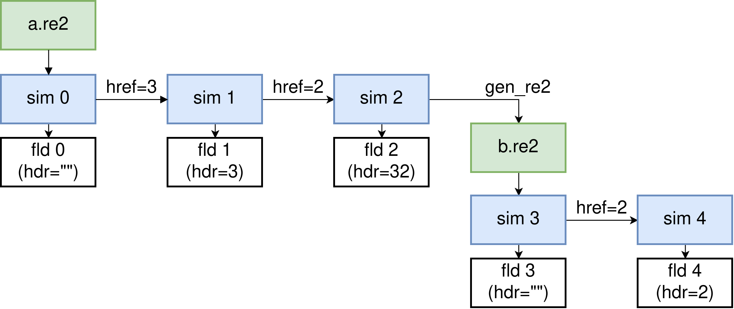
Fig. 3 Restart diagram for h-refinement. Starting from the top-left a.re2 (green), each simulation (blue) dumps a checkpoint file (white) whose header shows the stored h-schedule. After writing a new b.re2, the schedule is reset and older checkpoint files are no longer compatible.

Table 21 Supported restart scenarios

	Sim 1	Sim 2	Sim 3	Sim 4
fld 0	ok	ok	Not supported	Not supported
fld 1	ok	ok	Not supported	Not supported
fld 2	NA	ok	Not supported	Not supported
fld 3	NA	NA	ok	ok

Note

The h-refinement restart option can be combined with other restart options except int.

Miscellaneous Tips

Because high-order meshes place more degrees of freedom in each element, they typically use far fewer elements than lower-order CFD solvers. The quantity to monitor is therefore the total number of degrees of freedom, which depends on both the element count and the polynomial order. As a resource and performance metric, we use \(\mathrm{dof} = E N^3\), where \(E\) is the number of elements and \(N\) is the polynomial order.

Note

Each element contains \((N+1)^3\) GLL points, so the raw storage scales like \(\mathcal{O}(E (N+1)^3)\). However, many points are shared across element interfaces, so we define the effective number of degrees of freedom as \(\mathrm{dof} = E N^3\) for performance estimates.

Mesh refinement in higher-order finite elements can be performed in two ways:

• h-refinement: adding elements

• p-refinement: increasing the polynomial order of the elements

In practice, we rely on both to achieve an effective mesh resolution. Regions where the flow cross section changes abruptly, where separation occurs, or where the flow transitions (such as reactor plena) are good candidates for h-refinement. After obtaining converged results with a low polynomial order (e.g., N = 3), it is a good idea to switch to p-refinement and check whether the quantity of interest chosen for the mesh-refinement study continues to converge as the polynomial order increases. This process can be iterative: as one learns more about the flow physics, the need for additional h-refinement may become apparent when p-refinement alone fails to produce mesh convergence.

Note

For sufficiently smooth solutions, projecting onto piecewise polynomials of degree \(N\) on elements of size \(h\) in 3D yields a local truncation error of order \(\mathcal{O}(h^{N+1})\) under h-refinement (with \(N\) fixed). Since \(h \sim E^{-1/3}\) and \(|\Omega| \approx E h^3 = \mathcal{O}(1)\), the global \(L^2\)-error also scales as \(\mathcal{O}(h^{N+1})\).

When the solution is analytic on each element and the mesh is fixed, the coefficients in a modal Legendre polynomial expansion \(u(x) = \sum_{k=0}^\infty\ \hat{u}_k\ \phi_k(x)\) decay geometrically with respect to the polynomial degree. That is, there exist constants \(C>0\) and \(0 < \rho < 1\), independent of the mesh and \(N\), such that

\[|\hat{u}_k| \le C \,\rho^k \qquad \text{for all } k \ge 0.\]

The geometric decay of the modal coefficient implies that the trucation error decreases exponentially with \(N\), typically written as \(\|u - u_N\| \lesssim C \exp(-\alpha N)\) for some constants \(C, \alpha > 0\), in an appropiate norm (e.g., \(L^2\) or \(H^1\)).

High-order meshes can also tolerate element shapes that would be considered low quality in many low-order finite-element solvers. Depending on the physics, average aspect ratios of 20 or more can be acceptable. However, care must be taken to avoid overly small elements that are typical of low-order meshes, because NekRS will allocate N+1 Gauss–Lobatto–Legendre (GLL) nodes per element in each coordinate direction. This can easily lead to an excessive number of degrees of freedom. While the polynomial order can be reduced for such meshes (for example, when small geometric features impose element-size limitations), NekRS generally performs best when operating at higher polynomial orders (e.g., N >= 5).

Note

Combined with efficient matrix-free tensor-product operators of cost \(\mathcal{O}(E N^4)\) (without forming the full dof-by-dof system), high-order spectral elements typically offer better accuracy per dof and better scalability on modern distributed architectures that favor high compute intensity and data locality.

While increasing \(N\) generally improves accuracy per dof, using extremely high polynomial orders can become counterproductive:

• In finite-precision arithmetic, round-off error eventually dominates and limits the attainable accuracy.

• On GPUs, very large \(N\) increases register and shared-memory pressure, which can reduce occupancy and overall performance.

For these reasons, NekRS caps the polynomial order at \(N \le 10\), which provides a good balance between accuracy, robustness, and performance on modern architectures.

Note

For convection-dominated simulations, the timestep is constrained by the convective CFL condition. Because the minimum spacing of GLL points scales as \(\Delta x_{\min} \sim h / N^2\), mesh refinement (either decreasing \(h\) or increasing \(N\)) requires a corresponding reduction of \(\Delta t\) to maintain a fixed CFL number.

In practice, for LES and DNS where temporal resolution is critical, \(\Delta t\) is often chosen smaller than the CFL-limited value.