Models and Source Terms
With the exception of LES modelling, the User-Defined Host Functions (.udf) file in NekRS provides the necessary and sufficient interface to load most of the physics models (and postprocessing capabilities).
For instance, the RANS and lowMach compressible models available in nekRS are loaded by including corresponding header files in .udf and by calling the appropriate functions from the standard functions in .udf.
Appropriate boundary conditions for the momentum and scalar transport equations are specified in the okl block (or in the included .oudf file).
Further, any custom source terms that may need to be added to the momentum or scalar equations are also interfaced through the .udf file.
Before proceeding it is, therefore, highly recommended that users familiarize themselves with all components of .udf file.
Turbulence models
Large Eddy Simulation (LES)
Note
Pertinent example cases: turbPipe; turbChannel
In NekRS, the sub-grid scale dissipation for LES simulations is applied by means of a stabilizing filter, which drains energy from the solution at the lowest resolved wavelengths, effectively acting as a sub-grid scale model. A filter is necessary to run an LES turbulence model in NekRS and spectral methods in general, as they lack the numerical dissipation necessary to stabilize a so-called “implicit LES” method, which relies on a lack of resolution to provide dissipation.
The filter is constructed by means of a convolution operator applied on an element-by-element basis. Functions in the SEM are locally represented on each element as \(N^{th}\)-order tensor-product Lagrange polynomials in the reference element, \(\hat\Omega\equiv[-1,1]^3\). This representation can readily be expressed as a tensor-product of Legendre polynomials, \(P_k\). For example, consider
where \(u(x)\) is any polynomial of degree \(N\) on \([-1,1]\). As each Legendre polynomial corresponds to a wavelength on \([-1,1]\), a filtered variant of \(u(x)\) can be constructed from
By choosing appropriate values for the weighting factors, \(\sigma_k\), we can control the characteristics of the filter. In NekRS we select a filter cutoff ratio, \((N'+1)/(N+1)\), which can also be equivalently expressed as a number of filtered modes, \(N_{modes}=N-N'\). Weights are chosen as
to construct a low-pass filter. An example is shown below in Fig. 1. The signal produced by this filter would have the highest Legendre mode (shortest wavelength) completely removed with the next two highest modes significantly diminished. However, if the energy of the input signal is fully resolved on the first six modes, the filter would not affect the signal at all.
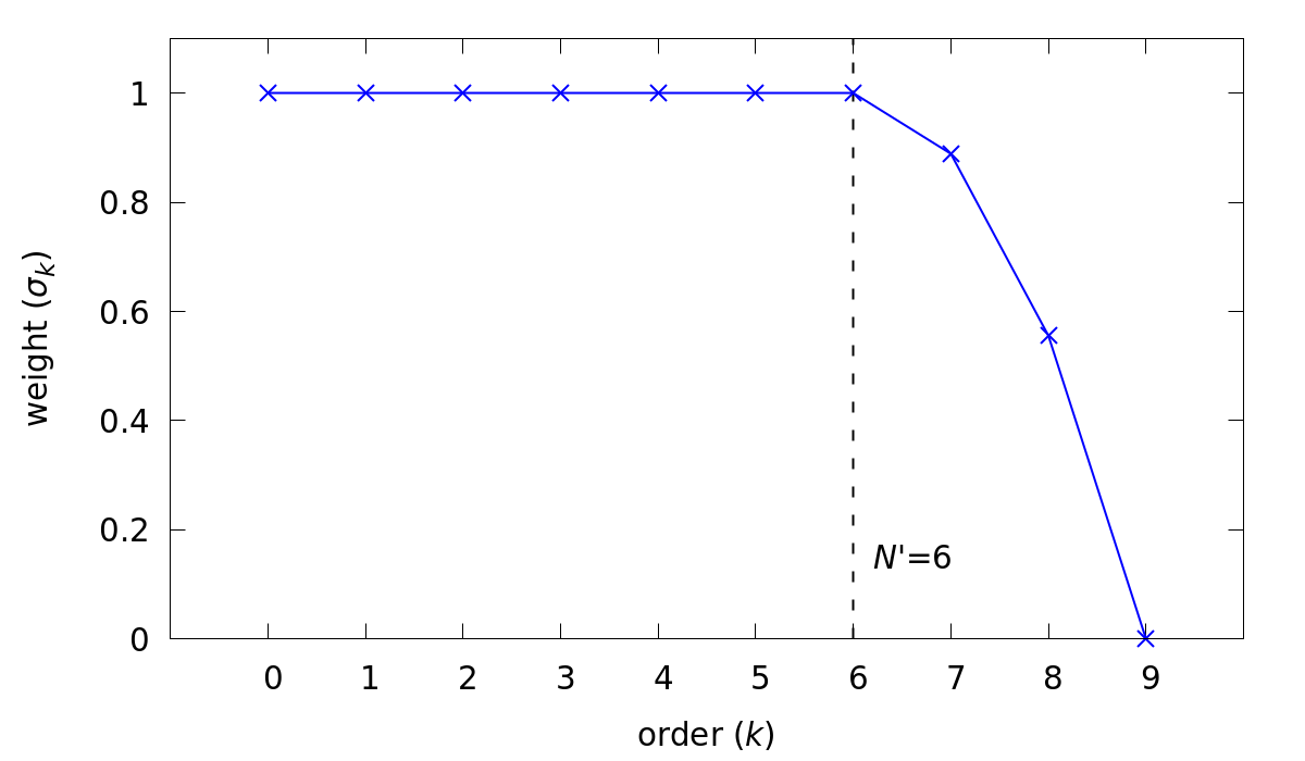
Fig. 1 Example of a strong low-pass filter.
To construct the filter on a three-dimensional element, we define \(F\) as the matrix operation that applies for this one-dimensional low-pass filter. From there, the convolution operator representing the three-dimensional low-pass filter, \((G*)\), on the reference element, \(\hat\Omega\), is given by the Kronecker product \(F \otimes F \otimes F\)
Warning
The filtered wavelengths depend on the local element size, so the filtering operation is NOT necessarily uniform across the domain.
High pass filter relaxation
The high-pass filter in NekRS is based on a method described by Stolz, Schlatter, and Kleiser [Stolz2005]. In the high-pass filter method, the convolution operator described above is used to obtain a low-pass filtered signal. The high-pass filter term is then constructed from the difference between the original signal and the low-pass filtered signal. For any scalar, this term has the form
where \(u\) is the original signal, \(\tilde u = G*u\) is the low-pass filtered signal, and \(\chi\) is a proportionality constant. In polynomial space, this term is only non-zero for the last few Legendre modes, \(k>N'\). It is subtracted from the RHS of the momentum, energy, and scalar transport equations, respectively
and acts to provide the necessary drain of energy out of the discretized system.
The high-pass filter can be invoked by setting the regularization=hpfrt key in the [GENERAL] section of the .par file.
The cutoff ratio used in the convolution operator, \((G*)\), is controlled by adding the nModes option to the regularization key.
The convolution operation used to construct the filtered signal, \(\tilde u\), completely removes the highest Legendre mode \(\sigma_N = 0\). The coefficients for the subsequent lower modes decrease parabolically until \(\sigma_{N'}=1\). This corresponds to a strong low-pass filtering operation, similar to the one shown in Fig. 1.
The overall strength of the high-pass filter is controlled by the proportionality coefficient, \(\chi\), which is set by adding the scalingCoeff option to the regularization key.
Typical values for this are \(5\le\chi\le10\), which drains adequate energy to stabilize the simulations.
The high-wavenumber relaxation of the high-pass filter model is similar to the approximate deconvolution approach [Stolz2001]. It is attractive in that it can be tailored to directly act on marginally resolved modes at the grid scale. The approach allows good prediction of transitional and turbulent flows with minimal sensitivity for model coefficients [Schlatter2006]. Furthermore, the high-pass filters enable the computation of the structure function in the filtered or HPF structure-function model in all spatial directions even for inhomogeneous flows, removing the arbitrariness of special treatment of selected (e.g. wall-normal) directions.
Generally recommended settings, specified in .par file, are as follows
[GENERAL]
regularization = hpfrt + nModes=1 + scalingCoeff=10
RANS models
Note
Pertinent example case: ktauChannel
Note
RANS model requires two passive scalar fields which must be specified in control parameters (.par) file.
For details on how to setup the .par file, refer to the section on .par file and also refer RANS Channel tutorial for specific example of .par file setup for RANS simulation
The essential routines for the RANS models in NekRS are available in the namespace in RANSktau.hpp.
The default RANS model in nekRS is the \(k\)-\(\tau\) model [Tombo2025].
Details on the formulation of the \(k\)-\(\tau\) can be found here.
To use the RANS model in nekRS, first declare the relevant scalar identifiers in .par file under the [GENERAL] card and include corresponding scalar solver cards
[GENERAL]
...

scalars = k, tau

...

[SCALAR K]
residualTol = 1e-8

[SCALAR TAU]
residualTol = 1e-8
Warning
The [SCALAR XX] cards for k and tau do not accept any transport properties for the corresponding equations.
They are specified internally, automatically, by the RANS solver.
Warning
nekRS assumes that the \(\tau\) field array always follows the TKE scalar field.
Thus, in the par file the order of k and tau in [GENERAL] card must be as shown above.
Next, add the necessary include file at the top of your .udf file:
#include "RANSktau.hpp"
The header file will make the required RANS subroutines accessible in the .udf file which add the necessary source terms for the \(k\) and \(\tau\) transport equations and modify the diffusion operator in the momentum equation.
Further, in the UDF_Setup() subroutine, add the following code snippet to initialize the RANS model,
void UDF_Setup()
{
  nrs->userProperties = &uservp;
  nrs->userSource = &userq;

  RANSktau::setup(nrs->scalar->nameToIndex.find("k")->second);

  //std::string model = "ktau";
  //std::string model = "ktausst";
  //std::string model = "ktausst+ddes";
  //std::string model = "ktausst+iddes";
  //RANSktau::setup(nrs->scalar->nameToIndex.find("k")->second, model);
}
RANSktau:: is the namespace declared in the header file RANSktau.hpp which contains all required RANS subroutine call definitions.
nrs->scalar->nameToIndex.find("k")->second returns the index of the scalar field where the turbulent kinetic energy, k, is stored.
The default RANS model in NekRS is the ktau model.
Thus, if no second argument is passed to RANSktau::setup() the standard ktau model is activated internally.
Alternatively, the user can explicity specify which RANS model to employ, as shown above.
Note
- The following RANS models are available in NekRS (names are not case sensitive):
KTAU : standard \(k\)-\(\tau\) model
KTAUSST: \(k\)-\(\tau\) shear-stress transport (SST) model
KTAUSST+DDES: \(k\)-\(\tau\) shear-stress transport (SST) delayed detached eddy simulation (DDES) model
KTAUSST+IDDES: \(k\)-\(\tau\) shear-stress transport (SST) improved delayed detached eddy simulation (IDDES) model
nrs->userProperties and nrs->userSource are the pointer variables to internal subroutines in nekRS which are used to define the user specified transport properties and source terms for the passive scalar equations, respectively.
As in the above code, these are assigned the pointers to uservp and userq routines which must be defined in the .udf file as follows,
void uservp(double time)
{
  RANSktau::updateProperties();
}

void userq(double time)
{
  RANSktau::updateSourceTerms();
}
The updateProperties() call computes the diffusion coefficients for the momentum and \(k\)-\(\tau\) equations (see RANS theory for details on RANS model equations), which are,
Note
updateProperties() also computes the eddy viscosity, \(\mu_t\), required in the above diffusion coefficients.
If the user desires to extract \(\mu_t\) array, say for post-processing purpose, it can be accessed as follows in the .udf file:
auto o_mue_t = RANSktau::o_mue_t();
The updateSourceTerms() call computes all source terms on the right hand side of the \(k\) and \(\tau\) transport equations, which are,
Note that the uservp and userq routines are called at each time step by the solver.
The above calls will, therefore, update the diffusion properties and source terms at each time step for all GLL points.
The final necessary step in the model setup for the \(k\)-\(\tau\) RANS model is the specification of the boundary conditions for the \(k\) and \(\tau\) transport equations.
As explained in the RANS theory section, the wall boundary condition for both \(k\) and \(\tau\) equations are zero.
These must be explicitly assigned in the okl block section of .udf file,
#ifdef __okl__

void udfDirichlet(bcData *bc)
{
  if(isField("scalar k") || isField("scalar tau")) bc->sScalar = 0;
}
isField() is used to identify the k and tau scalar fields and bc-sScalar is the pointer to the local GLL point on the wall.
Note
For wall resolved RANS simulations, the boundary conditions for both \(k\) and \(\tau\) transport equations are of Dirichlet type at the wall and equal to zero.
Warning
It is highly recommended to familiarize with okl block for proper boundary specification.
The above example assumes that the computational domain has no inlet boundaries. In case there are inlet boundaries present, they will also have Dirichlet type boundary condition for the \(k\) and \(\tau\) transport equations and it will be necessary to differentiate the value of \(k\) and \(\tau\) at the walls (zero) from those at the inlet (problem dependent).
This is done using bc->id identifier in the OKL block.
See boundary conditions section for usage details on how to specify boundary conditions.
Low-Mach Compressible Model
The low-Mach compressible model in NekRS is available through the routines defined in lowMach.hpp which must be included in the .udf file.
As default, this user guide assumes, and it is strongly recommended, that the low-Mach equations are solved in non-dimensional format.
However, appropriate instructions are included herein for dimensional solve.
For details on the low-Mach governing equation refer the theory section.
Get started with including the header file at the top of your case .udf file and declaring required global occa arrays,
#include "lowMach.hpp"

static deviceMemory<dfloat> o_beta;
static deviceMemory<dfloat> o_kappa;
o_beta is the global cache for storing the local isobaric expansion coefficients for all GLL points, while the o_kappa array stores the isothermal expansion coefficient.
Next, in the UDF_Setup() the following code snippet is required,
void UDF_Setup()
{
  nrs->userProperties = &uservp;
  nrs->userSource = &userq;
  nrs->userDivergence = &userqtl;

  o_beta.resize(nrs->fieldOffset);
  o_kappa.resize(nrs->fieldOffset);

  double gamma = 1.4;
  double alphaRef = (gamma - 1.0) / gamma;

  lowMach::setup(alphaRef, o_beta, o_kappa);
}
nrs->userProperties, nrs->userSource and nrs->userDivergence are internal nekRS pointers to provide an interface to user routines for specifying transport properties, source terms for scalar equation and (thermal) divergence for the right hand side of continuity equation, respectively.
uservp, userq and userqtl are the corresponding routines to be defined in the .udf file, described below.
The essential call in UDF_Setup() is lowMach::setup which initializes the required internal functions and arrays for the low-Mach compressible model.
It requires three arguments.
First argument, alpharef is the coefficient of the time derivative of the thermodynamic pressure, \(\frac{dp_t\dagger}{dt^\dagger}\), source term in the energy equation (see theory section).
Note
For real gases alpharef \(= \frac{p_0}{\rho_0 c_{p0} T_0}\), while for ideal gas assumption alpharef \(= \frac{\gamma_0 - 1}{\gamma_0}\), where \(\gamma_0\) is the isentropic expansion coefficient (1.4 in the above example).
Note
\(p_0\) and \(T_0\) are the pressure and temperature at reference conditions. \(\rho_0\), \(c_{p0}\) and \(\gamma_0\) are the density, specific heat capacity and isentropic expansion coefficient at reference conditions.
Warning
For solving the low-Mach equations in dimensional format, alpharef must be unity.
The remaining arguments to the lowMach::setup call are the pointers to the o_beta and o_kappa occa arrays.
Memory allocation for the o_beta and o_kappa arrays must be done using the resize functions and their extent must be equal to nrs->fieldOffset, which is the total number of GLL points.
The required transport properties and the expansion coefficient arrays are populated in the uservp routine,
void uservp(double time)
{
  fillProp(nrs->fluid->mesh->Nelements,
           nrs->fluid->fieldOffset,
           nrs->scalar->fieldOffset(),
           nrs->p0th[0],
           nrs->scalar->o_S,
           nrs->fluid->o_prop,
           nrs->scalar->o_prop,
           o_beta,
           o_kappa)
}
fillProp is a kernel which has to be defined in the okl block section of .udf file to populate the transport property arrays for the fluid (nrs->fluid->o_prop) and temperature (nrs->scalar->o_prop) equations and also the expansion coefficient arrays.
The details of the fillProp kernel are problem dependent.
An example for ideal gas assumption is shown below.
#ifdef __okl__

@kernel void fillProp(const dlong Nelements,
                      const dlong uOffset,
                      const dlong sOffset,
                      const dfloat p0th,
                      @restrict const dfloat *TEMP,
                      @restrict dfloat *UPROP,
                      @restrict dfloat *SPROP,
                      @restrict dfloat *BETA,
                      @restrict dfloat *KAPPA)
{
  for (dlong e = 0; e < Nelements; ++e; @outer(0)) {
    for (int n = 0; n < p_Np; ++n; @inner(0)) {
      const int id = e * p_Np + n;

      const dfloat rcpTemp = 1 / TEMP[id];
      UPROP[id + 0 * uOffset] = 1e-2;      // 1 / Re
      SPROP[id + 0 * sOffset] = 1e-2;      // 1 / Pe
      UPROP[id + 1 * uOffset] = p0th * rcpTemp;
      SPROP[id + 1 * sOffset] = p0th * rcpTemp;

      BETA[id] = rcpTemp;
      KAPPA[id] = 1 / p0th;
    }
  }
}
#endif
nrs->fluid->o_prop stores the fluid viscosity for all GLL points followed by density, while nrs->scalar->o_prop stores the diffusivity followed by the product of density and specific heat capacity at constant pressure.
Corresponding array offsets are, therefore, required by fillProp to identify the locations where each property is stored.
nrs->fluid->fieldOffset (uOffset) is the total number of GLL points in the fluid sub-domain, while the nrs->scalar->fieldOffset() (sOffset) returns the total number of GLL points in the temperature sub-domain.
Note
For a non-CHT case, nrs->fluid->fieldOffset will be equal to nrs->scalar->fieldOffset().
As mentioned earlier, in the above example fillProp kernel is specifically written for a calorically perfect ideal gas assumption with constant viscosity and thermal conductivity and with low-Mach equations solved in non-dimensional form.
Description of the property array specification depending on the case type is as follows (see theory section for description of notation),
Array Name |
Non-dimensional |
Dimensional |
||
Ideal Gas |
Real Gas |
Ideal Gas |
Real Gas |
|
|
\(\mu^\dagger/Re\) |
\(\mu^\dagger/Re\) |
\(\mu\) |
\(\mu\) |
|
\(\rho^\dagger = p_t^\dagger/T^\dagger\) |
\(\rho^\dagger\) |
\(\rho = p_t/R T\) |
\(\rho\) |
|
\(\lambda^\dagger/Pe\) |
\(\lambda^\dagger/Pe\) |
\(\lambda\) |
\(\lambda\) |
|
\(\rho^\dagger c_p^\dagger= p_t^\dagger c_p^\dagger/T^\dagger\) |
\(\rho^\dagger c_p^\dagger\) |
\(\rho c_p=p_tc_p/RT\) |
\(\rho c_p\) |
|
\(\beta^\dagger = 1/T^\dagger\) |
\(\beta_0 T_0 \beta^\dagger\) |
\(\beta = 1/T\) |
\(\beta\) |
|
\(\kappa^\dagger = 1/p_t^\dagger\) |
\(\kappa_0 p_0 \kappa^\dagger\) |
\(\kappa = 1/p_t\) |
\(\kappa\) |
Note
For real gases, the user can specify custom non-dimensional properties to the above arrays, depending on the equation of state.
Note
For an open system, the thermodynamic pressure is constant. Thus, \(p_t^\dagger=1\). Consequently, o_kappa array is constant and unity.
userq is the user routine to specify any problem dependent source term appearing in the temperature equation (e.g., volumetric source/sink term).
See the section on scalar source for details on the procedure for including any non-linear source terms in temperature equation.
For lowMach problems in a closed system and/or in a moving domain, it is necessary to add contribution of time derivative of thermodynamic pressure to the temperature equation.
A sub-routine is available in the lowMach:: namespace to add this contribution.
Include it as follows,
void userq(double time)
{
  lowMach::dpdt(nrs->scalar->o_EXT);
}
nrs->scalar->o_EXT is the internal occa array to store the non-linear source term for the scalar (temperature) equation.
The routine lowMach::dpdt will add the following contribution to this array,
nrs->scalar->o_EXT\(+=\)alpharef\(* \frac{dp_t}{dt}\)
where alpharef is the reference non-dimensional coefficient defined earlier in UDF_Setup().
Note
For open systems, lowMach::dpdt call is not required in userq. If called, it will merely add zero to nrs->scalar->o_EXT, since \(\frac{dp_t}{dt}=0\).
Further, lowMach system requires thermal divergence for the right hand side of continuity equation (see theory for details).
The routine to compute thermal divergence must be included in .udf as shown below,
void qtl(double time)
{
  lowMach::qThermalSingleComponent(time);
}
The above subroutine populates the nrs->fluid->o_div array which stores the local divergence.
Assuming constant viscosity and thermal conductivity, the divergence for real gas is,
nrs->fluid->o_div\(\rightarrow \frac{\beta_0 T_0 \beta_T^\dagger}{\rho^\dagger c_p^\dagger} \left(\nabla \cdot \frac{1}{Pe} \nabla T^\dagger + \dot{q}^\dagger + \frac{p_0}{\rho_0 c_{p0} T_0} \frac{d p_t^\dagger}{dt^\dagger}\right) - \kappa_0 p_0 \kappa^\dagger \frac{d p_t^\dagger}{d t^\dagger}\)
while for ideal gas it is,
nrs->fluid->o_div\(\rightarrow \frac{1}{\rho^\dagger c_p^\dagger T^\dagger} \left(\nabla \cdot \frac{1}{Pe} \nabla T^\dagger + \dot{q}^\dagger + \frac{\gamma_0-1}{\gamma_0} \frac{d p_t^\dagger}{dt^\dagger}\right) - \frac{1}{p_t^\dagger} \frac{d p_t^\dagger}{d t^\dagger}\)
Note
For closed system or moving domain problems, lowMach::qThermalSingleComponent also computes and updates the time derivative of thermodynamic pressure.
It is obtained by combining the continuity and energy equations and subsequent volume integral.
Thus, for real gas with constant viscosity and thermal conductivity we get,
\(\frac{d p_t^\dagger}{d t^\dagger} = \frac {1}{A} \left[-\int_\Gamma \vec{v}^\dagger \cdot \vec{n}_\Gamma d\Gamma + \beta_0 T_0 \int_\Omega \frac{\beta_T^\dagger}{\rho^\dagger c_p^\dagger} \left( \nabla \cdot \frac{1}{Pe} \nabla T^\dagger + \dot{q}^\dagger \right) d\Omega \right]\)
where, \(A = \int_\Omega \left(\kappa_0 p_0 \kappa^\dagger - \beta_0 T_0 \frac{\beta_T^\dagger}{\rho^\dagger c_p^\dagger} \frac{p_0}{\rho_0 c_{p0} T_0}\right) d\Omega\)
\(\Omega \rightarrow\) computational domain; \(\Gamma \rightarrow\) domain boundary; \(\vec{n}_\Gamma \rightarrow\) outward pointing normal.
Warning
In case of simulations involving multiple species (e.g., reactive flows), lowMach::qThermalSingleComponent is not valid.
A custom user routine will be required to account for divergence contribution from all species
Custom Source Terms
NekRS offers the user the option to add custom source terms in .udf file.
While the specific construction of the kernels for the user defined source terms will be problem dependent, the following section describes the essential components for building custom source terms for the momenutm and scalar transport equations.
Momentum Equation
Note
Pertinent example case: gabls1
In order to add source terms to the momentum or scalar equations declare a user defined function, (say) userSource, in .udf file and assign its pointer to the internal NekRS pointer used for identifying user defined function, nrs->userSource.
The nrs->userSource is initiated as a nullptr internally in NekRS.
The pointer must be assigned in UDF_Setup() routine.
The example below shows implementation of force term for buoyancy driven flow.
#ifdef __okl__
  @kernel void buoForce(const dlong N,
                        const dlong offset,
                        @restrict const dfloat *RHO,
                        @restrict const dfloat *g,
                        @restrict const dfloat *S,
                        @restrict dfloat *FU)
  {
    for (dlong n = 0; n < N; ++n; @tile(p_blockSize, @outer, @inner)) {
      if(n < N) {
        const dfloat rho = RHO[n];
        const dfloat fac = - p_Ri * rho * S[n];
        FU[n + 0 * offset] = fac * g[0];
        FU[n + 1 * offset] = fac * g[1];
        FU[n + 2 * offset] = fac * g[2];
      }
    }
  }
#endif

static occa::memory o_gvec;

void userSource(double time)
{
  auto mesh = nrs->fluid->mesh;

  auto o_rho = nrs->fluid->o_prop + nrs->fluid->fieldOffset;

  buoForce(mesh->Nlocal,
           nrs->fluid->fieldOffset,
           o_rho,
           o_gvec,
           nrs->scalar->o_S,
           nrs->fluid->o_EXT);
}

void UDF_LoadKernels(deviceKernelProperties& kernelInfo)
{
  kernelInfo.define("p_Ri") = 1.0; //Richardson Number
}

void UDF_Setup()
{
  nrs->userSource = &userSource;

  dfloat gvec[3] = {0.0, -1.0, 0.0};        //Unit gravity vector
  o_gvec = platform->device.malloc<dfloat>(3, gvec);
}
Note that the user defined source function, userSource, has one input argument i.e., current simulation time.
The custom force must be populated in the nrs->fluid->o_NLT occa array which is the designated internal occa array object for non-linear momentum source term.
The size of nrs->fluid->o_EXT is 3 * nrs->fieldOffset and, thus, it stores the three vector force components for all GLL points in the fluid domain.
The user defined okl kernel must be called in userSource for populating nrs->fluid->o_EXT.
The above example illustrates a forcing kernel constructed for buoyancy driven simulation in the Boussinessq limit.
It includes a simple kernel, buoForce, which assigns buoyancy acceleration along negative y-coordinate to demonstrate the indexing of nrs->fluid->o_EXT array.
o_gvec is the occa array initialized in UDF_Setup to specify the user desired normal vector of gravity (negative y in the above example).
p_Ri is the Richardson number which governs the scaling of the buoyancy force defined as a kernel directive in UDF_LoadKernels routine to make it available in the okl block.
o_rho defined in userSource is a temporary occa array variable that points to the internal property array nrs->fluid->o_prop.
Note the offset that must be specified, nrs->fieldOffset, to get the correct location of density.
For constructing more complicated custom forces, the user is encouraged to familiarize with okl block for further details on writing okl kernels.
Implicit Linearized Momentum Source
Note
Pertinent example case: hit
In addition to custom explicit force terms, as described above, NekRS also offers the option of adding implicit linearized custom force terms in .udf.
Implicit treatment of force terms can add more stability to the flow solver.
To implement linear force term start with assigning the pointer to nrs->fluid->userImplicitLinearTerm pointer object in UDF_Setup() routine,
deviceMemory<dfloat> implicitForcing(double time)
{
  auto mesh = nrs->fluid->mesh;

  poolDeviceMemory<dfloat> o_F(mesh->Nlocal);
  dfloat coeff = 1.0;
  platform->linAlg->fill(o_F.size(), -coeff, o_F);
  return o_F;
}

void UDF_Setup()
{
  nrs->fluid->userImplicitLinearTerm = &implicitForcing;
}
Note that the function object nrs->fluid->userImplicitLinearTerm (or implicitForcing) must have the return type deviceMemory<dfloat>, as shown above.
It takes an input argument, simulation time, which may be used to construct a time varying force term.
The above nominal example demonstrates the following forcing term added implicitly to the flow solver,
where -coeff factor is returned as an array, o_F, by the implicitForcing function.
poolDeviceMemory<dfloat> o_F(mesh->Nlocal) reserves memory for o_F from the internally available pool memory of size mesh->Nlocal (equal to the local number of GLL points).
Warning
The sign of the forcing coefficients must be opposite to the intended force term.
In the above example, the o_F array is constant.
However, it may be temporally or spatially varying array, depending on the application.
Note
nrs->fluid->userImplicitLinearTerm applies an isotropic coefficient to all components of the custom force.
Anisotropic implicit linear force terms are not supported.
Scalar Equations
Note
Pertinent example cases: lowMach
The procedure for implementing custom source term to the scalar equations (including temperature equation) is similar to momentum source term implementation.
Assign the pointer to the user defined source function, (say) userSource, to the internal NekRS pointer in UDF_Setup(),
void UDF_Setup()
{
  nrs->userSource = &userSource;
}
The internal NekRS occa memory for storing the custom (non-linear) source term for scalar equations is nrs->scalar->o_EXT.
This must be populated in the user defined userSource routine in .udf file.
A simple example is as follows,
#ifdef __okl__
  scalarSource(const dlong Nelements,
               @restrict const dfloat *X,
               @restrict dfloat *FS)
  {
    for (dlong e = 0; e < Nelements; ++e; @outer(0)) {
      for (int n = 0; n < p_Np; ++n; @inner(0)){
        const int id = e * p_Np + n;

        const dfloat x = X[id];
        FS[id] = x;
      }
    }
  }

#endif
void userSource(double time)
{
  for(int is = 0; is < nrs->scalar->NSfields; is++) {
    auto mesh = nrs->scalar->mesh(is);
    auto o_FS = nrs->scalar->o_EXT + nrs->scalar->fieldOffsetScan[is];
    scalarSource(mesh->Nelements,
                 mesh->o_x,
                 o_FS);
   }
}
The source terms for all passive scalar fields are in the contiguous array nrs->scalar->o_EXT.
Therefore, to index the location for any particular scalar field the appropriate offset must be specified.
The nrs->scalar->fieldOffsetScan[is] provides the offset for is scalar field which is used to fetch the pointer to the required memory address in nrs->scalar->o_EXT array (assigned to the temporary variable o_FS0).
nrs->scalar->NSfields is the total number of scalar fields.
An example of a custom okl kernel, scalarSource, is shown above which specifies the source term as a function of the local x-coordinate to all scalar fields.
More complex kernels can be constructed, as required, and applied only to specific scalars with proper indexing.