Theory

This page provides an overview of the governing equations available in NekRS. NekRS includes solvers for incompressible Navier-Stokes equation, a partially compressible low-Mach formulation, the Stokes equations, the \(k\)-\(\tau\) RANS equations and for general passive scalar advection-diffusion equation, including temperature equation.

Computational Approach

The spatial discretization in NekRS is based on the spectral element method (SEM) [Patera1984], which is a high-order weighted residual technique similar to the finite element method. In the SEM, the solution and data are represented in terms of \(N^{th}\)-order tensor-product polynomials within each of \(E\) deformable hexahedral (brick) elements. Typical discretizations involve elements of order upto \(N=10\) (corresponding to maximum of 1331 GLL points per element). Vectorization and cache efficiency derive from the local lexicographical ordering within each macro-element and from the fact that the action of discrete operators, which nominally have \(O(EN^6)\) nonzeros, can be evaluated in only \(O(EN^4)\) work and \(O(EN^3)\) storage through the use of tensor-product-sum factorization [Orszag1980]. The SEM exhibits very little numerical dispersion and dissipation, which can be important, for example, in stability calculations, for long time integrations, and for high Reynolds number flows. We refer to [Denville2002] for more details.

NekRS solves the unsteady incompressible two-dimensional, axisymmetric, or three-dimensional Stokes or Navier-Stokes equations with heat transfer in both stationary (fixed) or time-dependent geometry. It also solves the compressible Navier-Stokes in the Low Mach regime, and the magnetohydrodynamic equation (MHD). The solution variables are the fluid velocity \(\mathbf u=(u_{x},u_{y},u_{z})\), the pressure \(p\), the temperature \(T\). All of the above field variables are functions of space \({\bf x}=(x,y,z)\) and time \(t\) in domains \(\Omega_f\) and/or \(\Omega_s\) defined in Fig. 13. Additionally NekRS can handle conjugate heat transfer problems.

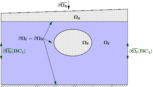
Fig. 13 Computational domain showing respective fluid and solid subdomains, \(\Omega_f\) and \(\Omega_s\). The shared boundaries are denoted \(\partial\Omega_f=\partial\Omega_s\) and the solid boundary which is not shared by fluid is \(\overline{\partial\Omega_s}\), while the fluid boundary not shared by solid \(\overline{\partial\Omega_f}\).

Incompressible Navier-Stokes Equations

The governing equations of incompressible flow in dimensional form are

\[\rho\left(\frac{\partial\mathbf u}{\partial t} +\mathbf u \cdot \nabla \mathbf u\right) = - \nabla p + \nabla \cdot \boldsymbol{\underline\tau} + \rho {\bf f} \,\, \quad \text{ (Momentum) }\]

where \(\boldsymbol{\underline\tau}=\mu[\nabla \mathbf u+\nabla \mathbf u^{T}]\) and \(\mathbf f\) is a user defined acceleration.

\[\nabla \cdot \mathbf u =0 \,\, \quad \text{ (Continuity) }\]

If the fluid viscosity is constant in the entire domain, the viscous stress tensor can be contracted using the Laplace operator. Therefore, one may solve the Navier–Stokes equations in either the full-stress formulation

\[\nabla \cdot \boldsymbol{\underline\tau}=\nabla \cdot \mu[\nabla \mathbf u+\nabla \mathbf u^{T}]\]

or the no-stress formulation

\[\nabla \cdot \boldsymbol{\underline\tau}=\mu\Delta \mathbf u\]

• Variable viscosity and RANS models require the full-stress tensor.

• Constant viscosity leads to a simpler stress tensor, which we refer to as the ‘no-stress’ formulation.

Non-Dimensional Navier-Stokes

Let us introduce the following non-dimensional variables \(\mathbf x^* = \frac{\mathbf x}{L}\), \(\mathbf u^* = \frac{u}{U}\), \(t^* = \frac{tU}{L}\), and \(\mathbf f^* =\frac{\mathbf f L}{U^2}\). Where \(L\) and \(U\) are the (constant) characteristic length and velocity scales, respectively. For the pressure scale we have two options:

• Convective effects are dominant i.e. high velocity flows \(p^* = \frac{p}{\rho_0 U^2}\)

• Viscous effects are dominant i.e. creeping flows (Stokes flow) \(p^* = \frac{p L}{\mu_0 U}\),

where \(\rho_0\) and \(\mu_0\) are constant reference values for density and molecular viscosity, respectively. For highly convective flows we choose the first scaling of the pressure and obtain the non-dimensional Navier-Stokes in the no-stress formulation:

\[\frac{\partial \mathbf{u^*}}{\partial t^*} + \mathbf{u^*} \cdot \nabla \mathbf{u^*}\ = -\nabla p^* + \frac{1}{Re}\Delta\mathbf u^* + \mathbf f^*.\]

For the full-stress formulation, we further introduce the dimensionless viscosity, \(\mu^*=\frac{\mu}{\mu_0}\), and obtain:

\[\frac{\partial \mathbf{u^*}}{\partial t^*} + \mathbf{u^*} \cdot \nabla \mathbf{u^*}\ = -\nabla p^* + \frac{1}{Re}\nabla \cdot \left[ \mu^* \left(\nabla\mathbf u^* + \nabla\mathbf u^{* T}\right)\right] + \mathbf f^*,\]

where \(\mathbf f^*\) is the dimensionless user defined forcing function. The non-dimensional number here is the Reynolds number \(Re=\frac{\rho_0 U L}{\mu_0}\).

Stokes Flow

In the case of flows dominated by viscous effects NekRS can solve the reduced Stokes equations

\[\rho\left(\frac{\partial \mathbf u}{\partial t} \right) = - \nabla p + \nabla \cdot \boldsymbol{\underline\tau} + \rho {\bf f} \,\, , \text{in } \Omega_f \text{ (Momentum) }\]

where \(\boldsymbol{\underline\tau}=\mu[\nabla \mathbf u+\nabla \mathbf u^{T}]\) and

\[\nabla \cdot \mathbf u =0 \,\, , \text{in } \Omega_f \text{ (Continuity) }\]

As described earlier, we can distinguish between the stress and non-stress formulation according to whether the viscosity is variable or not. The non-dimensional form of these equations can be obtained using the viscous scaling of the pressure.

Energy Equation

In addition to the fluid flow, NekRS offers the capability to solve the energy equation, where temperature is treated as a passive scalar for an incompressible flow.

\[\rho c_{p} \left( \frac{\partial T}{\partial t} + \mathbf u \cdot \nabla T \right) = \nabla \cdot (\lambda \nabla T) + \dot{q} \,\, \text{ (Energy) }\]

where, \(\lambda\) is the thermal conductivity and \(c_p\) is the specific heat at constant pressure.

Non-Dimensional Energy / Passive Scalar Equation

A similar non-dimensionalization as for the flow equations using the non-dimensional variables \(\mathbf x^* = \frac{\mathbf x}{L}\), \(\mathbf u^* = \frac{u}{U}\), \(t^* = \frac{tU}{L}\), \(T^*=\frac{T-T_0}{\delta T}\), and \(\lambda^*=\frac{\lambda}{\lambda_0}\) leads to

\[\frac{\partial T^*}{\partial t^*} + \mathbf u^* \cdot \nabla T^* = \frac{1}{Pe} \nabla \cdot \lambda^* \nabla T^* + q^* \,\, \text{ (Energy) }\]

where \(q^*=\frac{\dot{q} L}{\rho_0 c_{p_0} U \delta T}\) is the dimensionless user defined source term. The non-dimensional number here is the Peclet number, \(Pe=\frac{\rho_0 c_{p_0} U L}{\lambda_0}\).

Low-Mach Compressible Flow Equations

The low-Mach compressible equations are derived from the fully compressible Navier-Stokes equations by filtering the acoustic waves, obtained by splitting the pressure into thermodynamic, \(p_t\), and hydrodynamic components \(p_1\). The resulting low-Mach compressible governing equations, in dimensional form, are (for complete derivation refer [Tombo1997] or [Paulucci1982])

\[\begin{split}\nabla \cdot \mathbf{u} &= \beta_T \frac{D T}{D t} - \kappa \frac{D p_{t}}{D t} = Q\\ \rho \left(\frac{\partial \mathbf{u}}{\partial t} + \mathbf{u} \cdot \nabla \mathbf{u} \right) &= -\nabla p_1 + \nabla \cdot \mu \left(2 \boldsymbol{\underline{S}} - \frac{2}{3} Q \boldsymbol{\underline{I}} \right) + \rho \mathbf{f} \\ \rho c_p \frac{D T}{D t} &= \nabla \cdot \lambda \nabla T + \dot{q} + \frac{D p_t}{D t}\end{split}\]

where, \(\boldsymbol{\underline{S}} = \frac{1}{2}(\nabla \mathbf{u} + \nabla \mathbf{u}^T)\), \(Q\) is the divergence, \(\boldsymbol{\underline{I}}\) is the identity tensor and \(\dot{q}\) is the volumetric heat source term. Thermodynamic pressure is the leading order, spatially invariant, term in pressure expansion while hydrodynamic pressure is the first order term. \(\beta_T\) is the isobaric expansion coefficient and \(\kappa\) is the isothermal expansion coefficient,

\[\begin{split}\beta_T &= \frac{1}{\rho} \left.\frac{D \rho}{D t}\right|_p \\ \kappa &= \frac{1}{\rho} \left.\frac{D \rho}{D t}\right|_T\end{split}\]

Note

\(D \bullet/ Dt\) is the material derivative. Since \(p_t\) is spatially invariant, the convective component of its material derivative is zero. Therefore, \(D p_t/Dt = dp_t/dt\)

Note

For an open domain, the thermodynamic pressure is both spatially and temporally constant, i.e. \(dp_t/dt = 0\). This further simplifies the above equation system. However, for a closed system, the thermodynamic pressure, although uniform in space, is subject to changing temporally to enforce mass conservation.

The equation system above is not closed and an equation of state (EOS) is required to relate the density to the thermodynamic quantities, \(\rho = f(p_t,T)\). Further, dynamic viscosity and thermal conductivity also need to be provided by constitutive relations (e.g., Sutherland’s law for gases [Sutherland1893]).

Introducing the non-dimensional variables as follows,

\[\begin{split}\mathbf{u}^* = \frac{\mathbf{u}}{U}; \,\, T^* = \frac{T}{T_0}; \,\, \vec{x}^* = \frac{\vec{x}}{L};\,\, p_1^* = \frac{p_1}{\rho U^2};\,\, p_t^* = \frac{p_t}{p_0};\,\, t^* = \frac{t U}{L}; \vec{f}^* = \frac{\vec{f}}{f_0} \\ \rho^* = \frac{\rho}{\rho_0}; \,\, c_p^* = \frac{c_p}{c_{p0}}; \,\, \lambda^* =\frac{\lambda}{\lambda_0}; \,\, \mu^* = \frac{\mu}{\mu_0}; \,\, \beta_T^* = \frac{\beta_T}{\beta_0}; \,\, \kappa^* = \frac{\kappa}{\kappa_0}; \,\, \dot{q}^* = \frac{\dot{q} L}{\rho_0 c_{p0} T_0 U}\end{split}\]

the low-Mach governing equations are obtained as follows. The continuity equation:

\[\nabla \cdot \mathbf{u}^* = \beta_0 T_0 \beta_t^* \frac{D T^*}{D t^*} - \kappa_0 p_0 \kappa^* \frac{d p_t^*}{dt^*} = Q^*\]

mometum equation,

\[\rho^* \left(\frac{\partial \mathbf{u}^*}{\partial t^*} + \mathbf{u}^* \cdot \nabla \mathbf{u}^*\right) = - \nabla p_1^* + \nabla \cdot \frac{\mu^*}{Re} \left(2 \boldsymbol{\underline{S}}^* - \frac{2}{3} Q^* \boldsymbol{\underline{I}}\right) + \frac{1}{Fr} \rho^* \mathbf{f}^*\]

and energy equation,

\[\rho^* c_p^* \frac{D T^*}{D t^*} = \nabla \cdot \frac{\lambda^*}{Re Pr} \nabla T^* + \dot{q}^* + \frac{p_0}{\rho_0 c_{p0} T_0} \frac{d p_t^*}{d t^*}\]

where \(U\) and \(L\) are the characteristic velocity and length scales. \(f_0\) is reference magnitude of body force. \(p_0\) and \(T_0\) are the reference pressure and temperature, respectively, and \(\rho_0, \mu_0, c_{p0}, \lambda_0, \beta_0, \kappa_0\) are the corresponding fluid properties (density, dynamic viscosity, specific heat at contant pressure, conductivity, isobaric expansion coefficient and isothermal expansion coefficient, respectively) at reference conditions.

\(Re=\rho_0 U L/\mu_0\) is the Reynolds number, \(Pr = \mu_0 c_{p0}/\lambda_0\) and \(Fr=U^2/f_0 L\) are the Reynolds number, Prandtl number and Froude number, defined at reference conditions, respectively. The equations are closed by corresponding EOS in non-dimensional form, \(\rho^* = f(p_t^*,T^*)\). The above equations represent the lowMach equations in the most general form, applicable to real gases. Depending on the target application and associated assumptions, several simplifications to the equations are possible. In the subsequent section, we discuss the simplifications corresponding to the most commonly employed assumption, i.e., ideal gas assumption.

Low-Mach Equations with Ideal Gas Assumption

The EOS for an ideal gas is,

\[p_t = \rho R T; \,\, c_p-c_v = R \equiv \frac{R}{c_p} = \frac{\gamma - 1}{\gamma}\]

where \(R\) is the ideal gas constant, \(c_v\) is the specific heat at constant volume and \(\gamma = c_p/c_v\) is the isentropic expansion factor. In non-dimensional form, considering the properties at reference conditions for non-dimensionalization (i.e., \(p_0 = \rho_0 R T_0\) and \(\frac{R}{c_{p0}}= \frac{\gamma_0-1}{\gamma_0}\)), the EOS is simply written,

\[p_t^* = \rho^* T^*\]

The expansion coefficients, derived from the EOS, in non-dimensional form are,

\[\beta_T^* = \frac{1}{T^*} \,\, \kappa^* = \frac{1}{p_t^*}\]

The resulting governing equations for ideal gas assumption, thus, are,

\[\begin{split}\nabla \cdot \mathbf{u}^* &= \frac{1}{T^*} \frac{D T^*}{D t^*} - \frac{1}{p_t^*} \frac{d p_t^*}{dt^*} = Q^* \\ \rho^* \left(\frac{\partial \mathbf{u}^*}{\partial t^*} + \mathbf{u}^* \cdot \nabla \mathbf{u}^*\right) &= - \nabla p_1^* + \nabla \cdot \frac{\mu^*}{Re} \left(2 \boldsymbol{\underline{S}}^* - \frac{2}{3} Q^* \boldsymbol{\underline{I}}\right) + \frac{1}{Fr} \rho^* \mathbf{f}^* \\ \rho^* c_p^* \frac{D T^*}{D t^*} &= \nabla \cdot \frac{\lambda^*}{Re Pr} \nabla T^* + \dot{q}^* + \frac{\gamma_0-1}{\gamma_0} \frac{d p_t^*}{d t^*}\end{split}\]

Note

For a calorically perfect ideal gas, \(c_p\) will be constant and non-dimensional \(c_p^* = 1\).

Note

Another often used assumption is to consider dynamic viscosity and thermal conductivity independent of temperature (constant). Thus, \(\mu^*\) and \(\lambda^*\) will both be unity, further simplifying the above equations.

RANS Models

For turbulence modeling nekRS offers the two-equation \(k\)-\(\tau\) RANS model [Tombo2025] and its SST and DES variants [Kumar2024]. Linear two-equation RANS models rely on the Bousinessq approximation which relates the Reynolds stress tensor to the mean strain rate, \(\boldsymbol{\underline {S}}\), linearly through eddy viscosity. The time-averaged momentum equation is given as,

\[\begin{split}\rho \left(\frac{\partial \mathbf u}{\partial t} + \mathbf u \cdot \nabla \mathbf u \right) &= - \nabla p + \nabla \cdot \left[ (\mu + \mu_t) \left( 2 \boldsymbol{\underline S} - \frac{2}{3} Q \boldsymbol{\underline I}\right) \right] \\ \boldsymbol{\underline S} &= \frac{1}{2} \left( \nabla \mathbf u + \nabla\mathbf{u}^T \right)\end{split}\]

where \(\mu_t\) is the turbulent or eddy viscosity and \(\boldsymbol{\underline I}\) is an identity tensor. Currently, nekRS only supports incompressible flow where the divergence constraint, \(Q\), is zero,

\[Q = \nabla \cdot \mathbf u = 0\]

In two-equation models, the description of the local eddy viscosity is given by two additional transported variables, which provide the velocity and length (or time) scale of turbulence. The velocity scale is given by turbulent kinetic energy, \(k\), while the choice of the second variable, which provides the length or time scale, depends on the specific two-equation model used. In the \(k\)-\(\tau\) model, the second transported variable is \(\tau\), which is the inverse of the specific dissipation rate \(\omega\), and it provides the local time scale of turbulence.

The \(k-\tau\) model offers certain favorable characteristics over the \(k-\omega\) model [Wilcox2008], including bounded asymptotic behavior of \(\tau\) and its source terms and favorable near-wall gradients. These make it especially suited for high-order codes and complex geometries. It is, therefore, the preferred two-equation RANS model in NekRS. The \(k-\tau\) transport equations are,

\[\begin{split}\rho\left( \frac{\partial k}{\partial t} + \mathbf u \cdot \nabla k\right) & = \nabla \cdot (\Gamma_k \nabla k) + P_k - \rho \beta^* \frac{k}{\tau} \\ \rho\left( \frac{\partial \tau}{\partial t} + \mathbf u \cdot \nabla\tau\right) & = \nabla \cdot (\Gamma_\tau \nabla \tau) - \alpha \frac{\tau}{k}P_k + \rho \beta - 2\frac{\Gamma_\tau}{\tau} (\nabla \tau \cdot \nabla \tau) + C_{D_\tau}\end{split}\]

The diffusion terms are given by

\[\begin{split}\Gamma_k & = \mu + \frac{\mu_t}{\sigma_k} \\ \Gamma_\tau & = \mu + \frac{\mu_t}{\sigma_\tau}\end{split}\]

where, in the \(k-\tau\) model the eddy viscosity is given by,

\[\mu_t = \rho k \tau\]

The production term is given by

\[P_k = \mu_t\left( \boldsymbol{\underline S : \underline S} \right)\]

where “\(\boldsymbol :\)” denotes the double tensor contraction operator. The final term in the \(\tau\) equation is the cross-diffusion term, introduced by [Kok2000],

(6)\[C_{D_\tau} =(\rho \sigma_d \tau) \text{min}(\nabla k \cdot \nabla \tau,0)\]

The above term is especially relevant for external flows. It eliminates non-physical free-stream dependence of the near-wall \(\tau\) field (see [Tombo2025] for details).

All coefficients in the \(k-\tau\) model are identical to the standard \(k-\omega\) model [Wilcox2008], given as,

\[\beta = 0.0708; \,\, \beta^*=0.09; \,\, \alpha=0.52; \,\, \sigma_k= \frac{1}{0.6} \,\, \sigma_\tau=2.0; \,\, \sigma_d=\frac{1}{8}\]

Further theoretical and implementation details on the \(k\)-\(\tau\) model can be found in [Tombo2025].

Note

NekRS currently offers only wall resolved RANS models. The boundary condition for both \(k\) and \(\tau\) transport equations for wall resolved RANS are of Dirichlet type and equal to zero.