Conjugate Heat Transfer

In this tutorial, we simulate a simple quasi-2D Rayleigh-Benard convection (RBC) flow using NekRS’s conjugate heat transfer capability. The conjugate heat transfer capability solves the energy equation across both solid and liquid subdomains, while the incompressible Navier-Stokes equations are solved only in the liquid subdomain. In the case of RBC, this provides a continuous temperature profile through horizontal walls of finite thickness. The modeled case corresponds to a simplified version of simulations performed by Foroozani et al. [Foroozani2021].

If you are not familiar with NekRS, we strongly recommend that you begin with the Fully Developed Laminar Flow tutorial first! Get started with creating a directory, cht, to run this case in your favorite scratch folder.

cd $HOME/scratch
mkdir cht
cd cht

Governing Equations and Thermo-fluid Properties

This tutorial employs the Boussinesq approximation in the fluid, wherein density variations are assumed small and retained only in the buoyancy term. The resulting momentum and energy governing equations, written in non-dimensional form, for the fluid subdomain are:

\[ \begin{align}\begin{aligned}\frac{\partial \mathbf{u^*}}{\partial t^*} + \mathbf{u^*} \cdot \nabla \mathbf{u^*}\ = -\nabla p^* + \frac{1}{Re}\Delta\mathbf u^* - \mathbf{\hat{g}} \Theta Ri.\\\frac{\partial \Theta}{\partial t^*} + \mathbf u^* \cdot \nabla \Theta = \frac{1}{Pe} \nabla^2 \Theta\end{aligned}\end{align} \]

where, \(Ri = \frac{g \beta_T \Delta T L}{U^2}\) is the Richardson number, \(Re = \frac{\rho_0 U L}{\mu_0}\) is the Reynolds number and \(Pe = Re Pr\) is the Peclet number. \(Pr = \frac{\mu_0}{\rho_0 \alpha_0}\) is the Prandtl number of the fluid. \(\beta_T\) is the coefficient of thermal expansion, \(g\) is the gravitational acceleration and \(\rho_0\), \(\mu_0\) and \(\alpha_0\) are the reference fluid density, dynamic viscosity and thermal diffusivity, respectively. For natural convection simulations, the velocity scale is typically given by the buoyant velocity, i.e., \(U = \sqrt{g \beta_T L \Delta T}\). For the solid subdomain, the energy equation further simplifies since the convective term on the left hand side drops. Using consistent characteristic velocity and length scales, the governing equation in solid subdomain is

\[\frac{\partial \Theta}{\partial t^*} = \frac{\alpha_r}{Pe} \nabla^2 \Theta\]

where, \(\alpha_r\) is the ratio of solid to fluid thermal diffusivity. The non-dimensional properties selected for this tutorial are summarized in the following table:

Table 26 Non-dimensional fluid and thermal properties

Dimensionless number	Definition	Value
Rayleigh number, \(Ra\)	\(\frac{\rho_0 g \beta_T \Delta T L^3}{\mu_0 \alpha_0}\)	\(10^7\)
Prandtl number (fluid), \(Pr\)	\(\frac{\mu_0}{\rho_0 \alpha_0}\)	\(0.7\)
Richardson number, \(Ri\)	\(\frac{g \beta_T \Delta T L}{U^2}\)	\(1\)
Reynolds number, \(Re\)	\(\frac{\rho_0 U L}{\mu_0}\)	\(\sqrt{\frac{Ra}{Pr Ri}} \approx 3780\)
Peclet number, \(Pe\)	\(Re Pr\)	\(\approx 2646\)
Thermal diffusivity ratio, \(\alpha_r\)	\(\frac{\alpha_s}{\alpha_0}\)	\(0.2\)

Geometry and Boundary Conditions

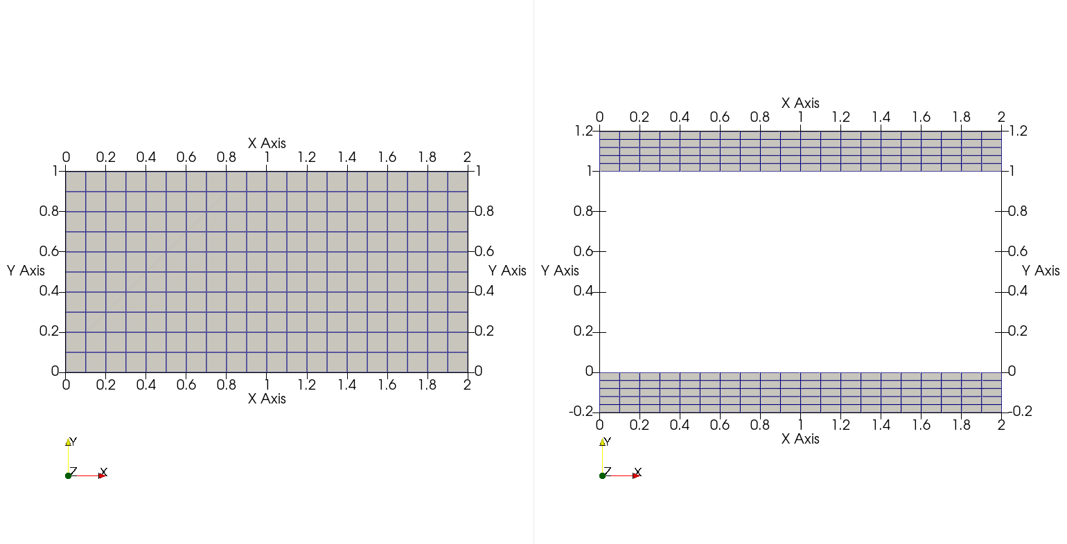
Fig. 9 Z-normal view of fluid (left) and solid (right) subdomains. Hexahedral elements from Gmsh are shown.

The fluid and solid subdomains for this example are as shown above. The base hexahedral mesh, generated using Gmsh, is also highlighted in the figure (see next section). Both fluid and solid domains are periodic in z-normal direction. Note that an arbitrary thickness of 0.1 is specified in the z-direction with 3 elements.

Note

NekRS mesh must have minimum of 3 elements across periodic boundaries.

All bounding surfaces of the fluid domain are wall boundaries (zero-slip), while the x-normal side walls are thermally insulated. In the solid domain, the x-normal walls are also insulated, while Dirichlet thermal boundary conditions are assigned on the top and bottom surfaces.

Mesh Generation

This tutorial uses mesh generated using the Gmsh tool. It is assumed that the user has successfully installed Gmsh on their system and has basic familiarity with generating meshes using this tool. Gmsh generates script files with the extension .geo which has the geometry and boundary ID information for the mesh. For the convenience of the user, the required .geo files for generating the meshes for this tutorial can be downloaded using the following links:

• fluid.geo

• solid.geo

Download the above files and save them in the working case directory - cht. The user must use these files to generate corresponding mesh files with .msh extension.

Tip

Typical steps to generate .msh file from .geo files are as follows:

• Open .geo file in Gmsh GUI

• Expand the Mesh tree in side navigation window in the GUI and generate mesh using the following steps:

  • Select 1D

  • Select 2D

  • Select 3D

  • Select Set Order 2

• Now save the mesh by selecting Export option from the File tab on top navigation bar.

  • A window will open where the name and location of mesh file can be assigned. The user must also assign the file extension. For this example, assign the name fluid.msh or solid.msh for the corresponding fluid.geo or solid.geo file that is currently open.

  • Another window will open that will prompt the user for mesh options:

    • For the format select Version 2 Binary

    • Ensure Save all elements is unchecked.

    • Ensure Save parameteric coordinates is unchecked

    • Select Ok

Following the above steps for both fluid.geo and solid.geo files will generate the mesh files fluid.msh and solid.msh files in the selected directory. The .msh files can also be directly downloaded using the following links:

• fluid.msh

• solid.msh

gmsh2nek is the tool to convert the Gmsh files into NekRS format. It is packaged and provided with Nek5000. For details on how to procure and compile gmsh2nek see Building the Nek5000 Tools. Run the gmsh2nek tool from the directory containing both fluid.msh and solid.msh files and follow the prompts as follows:

Enter mesh dimension: 3

Input fluid .msh file name: fluid
reading mesh file fluid.msh
total node number is         6027
total quad element number is          580
total hex element number is          600
total fluid hex number:          600

Entering the name of fluid mesh file, as shown above, prints information on number of elements and nodes in the mesh. Continuing further, the next prompt is specific to generating meshes for CHT cases. Specify the solid mesh as shown:

Do you have solid mesh ? (0 for no, 1 for yes) 1
Input solid .msh file name: solid
reading mesh file solid.msh
total node number is         6314
total quad element number is          700
total hex element number is          600

Next, gmsh2nek will provide information on the boundary surfaces and their corresponding IDs in the fluid and solid mesh files. There are declared in the .geo files and propogated by Gmsh in the .msh file. The boundary information in the fluid.msh and solid.msh as printed by gmsh2nek is as follows:

total hex number:         1200
reading mesh file fluid.msh
******************************************************
Fluid mesh boundary info summary
BoundaryName     BoundaryID
p1           1
p2           2
sideWalls           3
walls           4
******************************************************
reading mesh file solid.msh
******************************************************
Solid mesh boundary info summary
BoundaryName     BoundaryID
walls           4
p1          11
p2          12
bottomWall          13
topWall          14
sideWalls          15
******************************************************
performing non-right-hand check

Note

Make a note of the BoundaryID in the mesh files. These integer identifiers are required for setting up the NekRS case.

walls are the y-normal common surfaces interfacing the fluid and solid meshes.

Warning

Note that the common surfaces must be assigned identical BoundaryID in fluid and solid .geo files. The user must ensure this while generating geometry (.geo file) in Gmsh for CHT cases. Other surfaces can have arbitrary unique or identical BoundaryID depending on the intended boundary condition for the surfaces.

sideWalls are the x-normal walls in fluid and solid meshes and the topWall and bottomWall are the y-normal top and bottom surfaces in the solid mesh. p1 and p2 in the fluid and solid meshes are z-normal surfaces. In this example we will assign them periodic boundary condition, in order to setup a quasi-2D case with periodicity in z-direction. Note that while other boundary conditions are assigned in NekRS case files, the periodic boundary conditions must be established in the NekRS mesh file. gmsh2nek will prompt the user for setting up boundary condition, as shown below:

For Fluid domain
Enter number of periodic boundary surface pairs:
1
input surface 1 and  surface 2  Boundary ID
1 2

Enter, as shown above, the number of pairs of periodic boundaries in the mesh, 1 in this case. Following that, enter the corresponding boundary IDs in the fluid mesh for p1 and p2 surfaces - 1 2. gmsh2nek will confirm that periodicity was successfully established with the following message:

translation vector:    2.2204460492503131E-016     0.0000000000000000         0.10000000000000001
offset and normalize periodic face coordinates
bucket sorting to make index of each point
doing periodic check for surface           1
doing periodic check for surface           2
******************************************************
Please set boundary conditions to all non-periodic boundaries
in .usr file usrdat2() subroutine
******************************************************

Similary, establish periodicity for the z-surfaces in the solid domain:

For Solid domain
Enter number of periodic boundary surface pairs:
1
input surface 1 and  surface 2  Boundary ID
11 12
translation vector:   -2.2204460492503131E-016     0.0000000000000000        -0.10000000000000002
offset and normalize periodic face coordinates
bucket sorting to make index of each point
doing periodic check for surface          11
doing periodic check for surface          12
******************************************************
Please set boundary conditions to all non-periodic boundaries
in .usr file usrdat2() subroutine
******************************************************

Finally, gmsh2nek will ask the user the desired name of the NekRS mesh file. Specify cht as shown:

please give re2 file name:
cht

writing cht.re2
velocity boundary faces:          580
thermal boundary faces:         1280

gmsh2nek will now generate cht.re2 in the working directory and also print information on the total number of element faces in the fluid and solid mesh.

Control Parameters (.par file)

In the cht working directory, open file cht.par with your favorite text editor and specify NekRS parameters as follows (see details on Parameter File (.par)):

userSections = CASEDATA

[GENERAL] 
polynomialOrder = 5
stopAt = endTime
endTime = 200.0
dt = targetcfl=1.0+initial=1e-3
timeStepper = tombo2

checkPointControl = simulationTime
checkpointInterval = 10.0

scalars = temperature

[MESH]
boundaryIDMap = 3, 4, 1, 2, 13, 14, 15, 11, 12                    #Maps ids to 1, 2, 3...
boundaryIDMapFluid = 3, 4, 1, 2               #for CHT case only  #Maps ids to 1, 2, 3...

[FLUID PRESSURE]
residualTol = 1e-06

[FLUID VELOCITY]
boundaryTypeMap = zeroDirichlet, zeroDirichlet, none, none
residualTol = 1e-08
rho = 1.0
mu = 1.0/3780.0                               # 1 / Re 

[SCALAR TEMPERATURE]
boundaryTypeMap = zeroNeumann, none, none, none, udfDirichlet, udfDirichlet, zeroNeumann, none, none
residualTol = 1e-08
mesh = fluid+solid                            #for CHT case only

transportCoeff = 1.0                          #rho*cp of fluid for dimensional case
transportCoeffSolid = 1.0                     #rho*cp of solid for dimensional case

diffusionCoeff = 1.0/2646.0                   #1 / Pe          #thermal conductivity of fluid for dimensional case
diffusionCoeffSolid = 0.2/2646.0              #alpha_r / Pe    #thermal conductivity of solid for dimensional case

[CASEDATA]
Tboundary = 1.0
Richardson = 1.0

In the [GENERAL] section specify the scalar identifier for temperature field using scalars = temperature key and value. A conjugate heat transfer case has some important distinctions in the .par file as compared to a more typical case with fluid only mesh. Particularly, the boundary surfaces of the CHT mesh must be carefully assigned under the [MESH] section using the boundaryIDMapFluid key, in addition to the boundaryIDMap key.

Note

For a non-CHT case the mesh surfaces are defined using the boundaryIDMap key. boundaryIDMapFluid is only required for a CHT case to explicitly specify the fluid subdomain mesh IDs.

The sequence of comma-separated integer values assigned to the boundaryIDMap or boundaryIDMapFluid correspond to the mesh boundary IDs specified in the third-party mesher, Gmsh in this case. The boundary IDs were detailed in the previous section and can be recorded from the gmsh2nek output. The mesh boundary IDs may be specified to these keys in any arbitrary sequence, but the corresponding boundary conditions specified in specific field sections using boundaryTypeMap must be consistent with the sequence of mesh surface IDs. As defined in previous section the fluid subdomain mesh has periodic z-surfaces 1 and 2, x-normal side walls with ID 3 and y-normal walls with ID 4. The corresponding boundary condition in the [FLUID VELOCITY] section specified with boundaryTypeMap is zeroDirichlet for surface IDs 3 and 4 and none for periodic surfaces 1 and 2.

The user should take note that the boundaryTypeMap in [SCALAR TEMPERATURE] section specifies boundary conditions for all mesh surfaces, including fluid and solid subdomains. The solid-fluid interface surface, which has the ID 4 as assigned in Gmsh (see previous section), has the value none. Similarly, the periodic mesh surfaces 1,2 and 11,12 also have the value none.

Note

Periodic or internal surface must be assigned the value none in boundaryTypeMap.

The side walls in both fluid (3) and solid (15) subdomains are thermally insulated and assigned the zeroNeumann value, while the top and bottom surfaces of the solid domain have Dirichlet thermal boundary conditions, identified with udfDirichlet value.

Another important distinction between a CHT case and fluid only mesh case is in the material property specification for the scalar field in .par file. The properties for this case are listed in this table. In [SCALAR TEMPERATURE] it is required to distinguish the mesh for the solution of the scalar field with mesh = fluid+solid key, which instructs the solver to solve the TEMPERATURE field in both fluid and solid subdomains. The material properties in the fluid subdomain are specified with the usual keys, transportCoeff and diffusionCoeff for volumetric heat capacity \((\rho c_p)\) and thermal conductivity \((\lambda)\), respectively. Corresponding properties in the solid subdomain are assigned with the keys transportCoeffSolid and diffusionCoeffSolid.

Note

Since this simulation is setup in non-dimensional format:

• transportCoeff = 1 (\(\rho c_p\) of fluid for dimensional case)

• transportCoeffSolid = 1 (\(\rho c_p\) of solid for dimensional case)

• diffusionCoeff = 1 / Pe (\(\lambda\) of fluid for dimensional case)

• diffusionCoeffSolid = \alpha_r / Pe (\(\lambda\) of solid for dimensional case)

Tip

The above method for property specification in .par file is valid if properties in the subdomains are spatially and temporally constant. In case the user wants varying properties, they must be specified in .udf file. See Conjugate Heat Transfer for details.

This case also uses some user defined parameter, specified in userSections - [CASEDATA] which are used for setting up boundary and initial conditions in .udf file.

• Tboundary is used to specify Dirichlet boundary condition

• Richardson is used to specify Richardson number

Remaining entries in the .par file are similar to a typical fluid only case. For more details see Parameter File (.par).

User-Defined Host Functions File (.udf)

Loading User Parameters

Begin with opening cht.udf file in your favorite editor and declaring some global variables we will use in the .udf file:

static dfloat Tb;
static dfloat Ri;
static occa::memory o_gvec;

In UDF_Setup0 routine read the values from .par file into these global variables

void UDF_Setup0(MPI_Comm comm, setupAide &options)
{
  platform->par->extract("casedata","Tboundary",Tb);
  platform->par->extract("casedata","Richardson",Ri);
}

As mentioned earlier, Tboundary is the absolute of Dirichlet temperature value we will define at top and bottom solid mesh surfaces and Richardson is the Richardson number used to scale the buoyancy force. Their values from .par file are store in Tb and Ri global variables, as shown above. o_gvec is a global OCCA array defined to store the unit gravitational force vector. Since, we also intend to make Tb and Ri values available in OKL block, also load these into kernel macros p_Tb and p_Ri in UDF_LoadKernels function as shown:

void UDF_LoadKernels(deviceKernelProperties& kernelInfo)
{
  kernelInfo.define("p_Tb") = Tb;
  kernelInfo.define("p_Ri") = Ri;
}

Initializations

Next, add UDF_Setup routine as follows:

void UDF_Setup()
{
  nrs->userSource = &userSource;

  dfloat gvec[3] = {0.0, -1.0, 0.0};        //Unit gravity vector
  o_gvec = platform->device.malloc<dfloat>(3, gvec);

  if (platform->options.getArgs("RESTART FILE NAME").empty()) {
    {
      auto& fluid = nrs->fluid;
      auto mesh = fluid->mesh;
      auto [x, y, z] = mesh->xyzHost();
      std::vector<dfloat> U(mesh->dim * fluid->fieldOffset, 0.0);
      for(int n = 0; n < mesh->Nlocal; n++) {
        U[n + 0 * fluid->fieldOffset] = 0.0;
        U[n + 1 * fluid->fieldOffset] = 0.0;
        U[n + 2 * fluid->fieldOffset] = 0.0;
      }
      fluid->o_U.copyFrom(U.data(), U.size());
    }

    {
      auto& scalar = nrs->scalar;
      auto mesh = scalar->mesh("temperature");
      auto [x, y, z] = mesh->xyzHost();
      std::vector<dfloat> T(mesh->Nlocal);

      for(int n = 0; n < mesh->Nlocal; n++) {
        T[n] = 0.0; 

        if(y[n] < 0.0) T[n] = Tb;
        if(y[n] > 1.0) T[n] = -Tb;
      }
      scalar->o_solution("temperature").copyFrom(T.data(), T.size());
    }
  }
}

The internal NekRS pointer, nrs->userSource, is assigned to a user-defined routine in .udf - userSource. It is detailed in the next sub-section. The gravitational vector is defined next and populated in the o_gvec OCCA array. o_gvec is allocated using platform->device.malloc<dfloat>. Note that the force is acting in the negative y-direction.

The next task is to assign initial conditions, which is done in an if block which checks for the condition if the case is being restarted, as shown above. It is important to note in the code above that the velocity components and temperature are initialized in separate blocks (enclosed with {}). This is because the mesh objects for the fluid and solid subdomains are different. When initializing the velocity components the fluid->mesh object is used, whereas for temperature initialization the scalar->mesh("temperature") object must be used. Subsequently the mesh coordinates can be procured into host arrays using a convenient routine, mesh->xyzhost(). Loop over mesh->Nlocal can then be used to fill out initial condition for velocity or temperature into temporary host container arrays U and T. As shown above, assign zero temperature value to the fluid subdomain, Tb to the bottom part of solid subdomain and -Tb to the top part. Finally, copy the initial values from host container arrays, U and T, to field OCCA arrays, fluid->o_U and scalar->o_solution("temperature"), using copyFrom routine.

Custom Buoyancy Source

The userSource routine is as follows and it is used to assign the buoyancy force term to the momentum equation for this case.

void userSource(double time)
{
  auto mesh = nrs->fluid->mesh;

  auto o_rho = nrs->fluid->o_prop.slice(1 * nrs->fluid->fieldOffset);

  auto o_temp = nrs->scalar->o_solution("temperature");

  buoForce(mesh->Nlocal,
           nrs->fluid->fieldOffset,
           o_rho,
           o_gvec,
           o_temp,
           nrs->fluid->o_EXT);
}

buoForce is a custom kernel function, detailed in next section, which takes fluid density (o_rho), gravity vector (o_gvec) and temperature (o_temp) to construct the buoyancy force populated in fluid->o_EXT, which is the explicit forcing array for the momentum equation.

Boundary Conditions and Buoyancy Force (okl block)

Dirichlet boundary conditions for temperature are assigned within the udfDirichlet kernel function as shown below. It is important to note that the sequence of mesh IDs specified in .par file using the boundaryIDMap or boundaryIDMapFluid key are mapped internally in ascending integer sequence starting from 1. Thus, the bottom surface with mesh ID 13 is mapped to bc->id = 5, while the top surface with mesh ID 14 is mapped to bc->id = 6. These can be used to identify the boundary surface in udfDirichlet. As shown, the bottom surface is assigned the temperature value of p_Tb, while the top surface -p_Tb.

#ifdef __okl__

void udfDirichlet(bcData *bc)
{
  if(isField("scalar temperature")) {
    if(bc->id == 6) bc->sScalar = -p_Tb;           //top surface
    if(bc->id == 5) bc->sScalar = p_Tb;            //bottom surface
  }
}

@kernel void buoForce(const dlong N,
                      const dlong offset,
                      @restrict const dfloat *RHO,
                      @restrict const dfloat *g,
                      @restrict const dfloat *S,
                      @restrict dfloat *FU)
{
  for (dlong n = 0; n < N; ++n; @tile(p_blockSize, @outer, @inner)) {
    if(n < N) {
      const dfloat rho = RHO[n];
      const dfloat fac = - p_Ri * rho * S[n];
      FU[n + 0 * offset] = fac * g[0];
      FU[n + 1 * offset] = fac * g[1];
      FU[n + 2 * offset] = fac * g[2];
    }
  }
}
#endif

The buoForce is a custom kernel included in the OKL block to fill buoyancy force in the explicit forcing array for momentum equation, i.e., nrs->o_fluid->o_EXT. The magnitude of forcing term, as in momentum equation, is \(Ri \Theta\).

Note

Note, density array RHO has unit values for the non-dimensional case. It not necessarily needed for current setup. The array is passed to buoForce kernel in the above setup for generality. It will be needed for dimensional case.

UDF_ExecuteStep

No operations are performed in the UDF_ExecuteStep for this tutorial. However, it is a necessary routine. Thus, include it as shown.

void UDF_ExecuteStep(double time, int tstep)
{
}

Compilation and Running

All required case files for RANS wall-resolved channel simulation can be downloaded using the links below:

• cht.re2

• cht.par

• cht.udf

If for some reason you encountered an insurmountable error and were unable to generate any of the required files, you may use the provided links to download them. Now you can run the case.

$ nrsbmpi cht 4

The above command will launch an MPI jobs on your local machine using 4 ranks. The output will be redirected to logfile.

Results

Once execution is completed your directory should now contain multiple checkpoint files that look like this:

cht0.f00000
cht0.f00001
...

The preferred mode for data visualization with NekRS is to use Visit or Paraview. This requires generating a metadata file with nrsvis. It can be run with

$ nrsvis cht

to obtain a file named cht.nek5000. This file can be opened with either Visit or Paraview. In the viewing window, the velocity magnitude and temperature fields can be visualized. The image below shows the contour profiles at steady state.

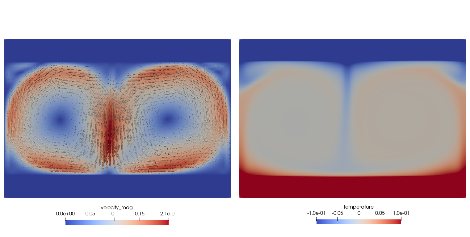
Fig. 10 Steady-state velocity magnitude (left) and temperature (right) contours.