Fully Developed Laminar Flow

In this tutorial we will be building a case that involves incompressible laminar flow in a channel with a constant heat flux applied. This case uses air as a working fluid and will be simulated using fully dimensional quantities. A diagram of the case is provided in Fig. 4 and the necessary case parameters are provided in Table 25. Note that round numbers have been selected for the fluid properties and simulation parameters for the sake of simplicity.

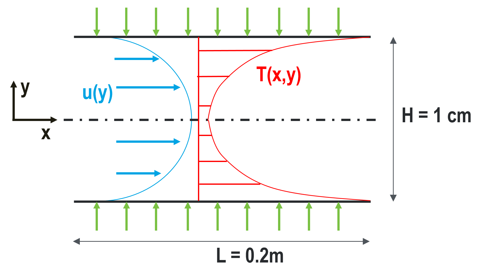
flow diagram — Fig. 4 Diagram describing the case setup for fully developed laminar flow in a channel.

Table 25 Fluid properties and simulation parameters
Parameter name	variable	value
channel height	\(H\)	1 cm
channel length	\(L\)	20 cm
mean velocity	\(U_m\)	0.5 m/s
heat flux	\(q''\)	300 W/m²
inlet temperature	\(T_{in}\)	10 C
density	\(\rho\)	1.2 kg/m³
viscosity	\(\mu\)	0.00002 kg/m-s
thermal conductivity	\(\lambda\)	0.025 W/m-K
specific heat	\(c_p\)	1000 J/kg-K

This case has analytic solutions to the momentum and energy equations which makes it easy to confirm if the problem is setup correctly. These expressions will be used to test the accuracy of the solution.

(1)\[u(y) = \frac{3}{2} U_m \left( 1 - 4\left(\frac{y}{H}\right)^2\right)\]

(2)\[T(x,y)-T_b(x) = \frac{q'' H}{2\lambda}\left( 3\left(\frac{y}{H}\right)^2 - 2\left(\frac{y}{H}\right)^4-\frac{39}{280}\right)\]

where the bulk temperature is given by the expression

\[T_b(x) = \left(\frac{2q''}{U_m \rho c_p H}\right)x + T_{in}\]

Before You Begin

This tutorial assumes that you have installed NekRS and have setup your PATH environment to point to installation directory. Instructions for installation and setting environment can be found in Quickstart guide.

Before running the case, you will need the mesh generation tool genbox. These tools are not packaged with NekRS but are available with Nek5000. Please follow the instructions in the Building the Nek5000 Tool Scripts section to obtain and build this tool.

Mesh Generation

This tutorial uses a simple 3D cuboid box mesh generated by genbox. To create the input file for genbox, copy the following script and save the file as fdlf.box.

-3                     spatial dimension (will create box.re2)
2                      number of fields
#
#    comments: periodic laminar flow
#
#========================================================
#
Box                                       fdlf
-50 -5 -3                                 Nelx Nely Nelz
0.0 0.2 1.0                               x0 x1 ratio
0.0 0.005 0.7                             y0 y1 ratio
0.0 0.1 1.0                               z0 z1 ratio
v  ,O  ,SYM,W  ,P  ,P                     Velocity BCs
t  ,O  ,I  ,f  ,P  ,P                     Temperature BCs

For this mesh we are specifying 50 uniform elements in the stream-wise (\(x\)) direction, 5 uniform elements in the span-wise (\(y\)) direction, and 3 uniform element in \(z\)-direction.

Note

NekRS can only solve 3D problems, therefore the mesh has 3 elements in the z-direction with periodic boundary condition. At least 3 mesh layers are required to correctly construct the mesh connectivity array in NekRS.

The velocity boundary conditions in the x-direction are a standard Dirichlet velocity boundary condition at \(x_{min}\) and an open boundary condition with zero pressure at \(x_{max}\). In the y-direction the velocity boundary conditions are a symmetric boundary at \(y_{min}\) and a wall with no slip condition at \(y_{max}\). In the z-direction there is a periodic velocity boundary condition at both \(z_{min}\) and \(z_{max}\).

The temperature boundary conditions in the x-direction are a standard Dirichlet boundary condition at \(x_{min}\) and an outflow condition with zero gradient at \(x_{max}\). In the y-direction the temperature boundary conditions are an insulated condition with zero gradient at \(y_{min}\) and a constant heat flux at \(y_{max}\). The z direction boundary conditions are periodic at both \(z_{min}\) and \(z_{max}\).

Note that the boundary conditions specified with lower case letters must have values assigned in relevant functions in the udf file, which will be shown later in this tutorial (see Boundary Conditions). Now we can generate the mesh with:

$ genbox

When prompted provide the input file name, which for this case is fdlf.box. The tool will produce binary mesh and boundary data file box.re2 which should be renamed to fdlf.re2:

$ mv box.re2 fdlf.re2

Tip

If genbox cannot be located by your shell, check to make sure the Nek5000/bin directory is in your path. For help see Nek5000 setting PATH. A detailed explaination of the Nek5000 box format can be found Nek5000 Doc genbox

Control parameters file (.par)

The control parameters for any case are given in the par file. For this case, create a new file called fdlf.par with the following:

userSections = CASEDATA

[GENERAL]
polynomialOrder = 5
stopAt = endTime
endTime = 1.0
dt = 1e-04
timeStepper = tombo2

checkpointControl = simulationTime 
checkpointInterval = 0.2

scalars = temperature

[PROBLEMTYPE]
equation = navierStokes

[FLUID PRESSURE]
residualTol = 1e-04

[FLUID VELOCITY]
residualTol = 1e-06
rho = 1.2
viscosity = 0.00002 

[SCALAR TEMPERATURE]
residualTol = 1e-06
transportCoeff = 1200.0
diffusionCoeff = 0.025 

[CASEDATA]
UMEAN = 0.5
HEATFLUX = 300.0
TINLET = 10
HEIGHT = 0.01

The constant fluid and temperature properties, as listed in Table 25 are specified under the [FLUID VELOCITY] and [SCALAR TEMPERATURE] sections, respectively.

Note

Any passive scalar being solved for must be assigned a string identifier in [GENERAL] section, as shown above, using the scalars key.

rho and viscosity keys correspond to the fluid density and dynamic viscosity, while the transportCoeff and diffusionCoeff corresponds to volumetric heat capacity, \(\rho c_p\), and thermal conductivity, \(k\), respectively.

The required values for the initial and boundary conditions specified by lower case letters in the .box file are defined here as part of the [CASEDATA] section, as shown above. This optional section must be explicity identified in .par file using the userSections key. This provides an easy way of passing data to NekRS that can later be used throughout the .udf file where the conditions will later be set. Additionally, like all values specified in the .par file, they can be changed without the need to recompile NekRS.

The above case is run with a polynomial order of 5 and upto \(t=1s\), as specified using endTime key. Details on the other keys in the .par can be found here.

User-Defined Host Functions File (.udf)

The user-defined host functions file implements various subroutines, including initial and boundary conditions, to allow the user to interact with the solver. Get started with creating a new file called fdlf.udf and defining the following sections:

Loading user parameters

Define global variables to store the mean velocity, heat flux, inlet temperature and channel height defined in the [CASEDATA] section of the .par file,

static dfloat umean;
static dfloat heatflux;
static dfloat tinlet;
static dfloat height;

The static keyword in c++ instructs the compiler to make the variable visible and accessible only within the source file where it is defined, in this case fdlf.udf file. The values are loaded inside the UDF_Setup0 function as follows,

void UDF_Setup0(MPI_Comm comm, setupAide &options)
{
  platform->par->extract("casedata", "umean", umean);
  platform->par->extract("casedata", "heatflux", heatflux);
  platform->par->extract("casedata", "tinlet", tinlet);
  platform->par->extract("casedata", "height", height);
}

Three parameters are taken by platform->par->extract function, viz., the user section name, key defined by user and the variable where the value from .par file is stored, respectively.

Note

The variables defined in user section in .par file, in this case [CASEDATA] section, are case insensitive.

To also make these variables available in device kernels in OKL block, where boundary conditions are assigned, the UDF_LoadKernels function is used to define device specific variables as follows,

void UDF_LoadKernels(deviceKernelProperties& kernelInfo)
{
  kernelInfo.define("p_umean") = umean;
  kernelInfo.define("p_hflux") = heatflux;
  kernelInfo.define("p_tinlet") = tinlet;
  kernelInfo.define("p_height") = height;
}

where kernelInfo.define(p_xxxx) function declares the device specific variable p_xxxx.

Note

Following NekRS source code convention, user specified global device variables should start with p_.

Initial Conditions

The initial conditions for the case must be specified in the UDF_Setup routine. For this case, we specify them as follows,

void UDF_Setup()
{
  auto mesh = nrs->meshV;

  std::vector<dfloat> U(mesh->dim * nrs->fluid->fieldOffset, 0.0);
  std::vector<dfloat> temp(mesh->Nlocal, 0.0);

  if (platform->options.getArgs("RESTART FILE NAME").empty()) {
    for(int n = 0; n < mesh->Nlocal; n++) {
      U[n + 0 * nrs->fluid->fieldOffset] = umean;
      U[n + 1 * nrs->fluid->fieldOffset] = 0;
      U[n + 2 * nrs->fluid->fieldOffset] = 0;
      temp[n] = tinlet;
    }
    nrs->fluid->o_U.copyFrom(U.data(), U.size());
    nrs->scalar->o_solution("temperature").copyFrom(temp.data(), temp.size()); 
  }
}

nrs->meshV is the pointer that references the mesh object for the nrs (or fluid) solver. U and temp are temporary dynamically allocated arrays on host, used to store the initial conditions. mesh->ndim is the number of spatial dimensions (always equal to 3) and nrs->fluid->fieldOffset equals the number of local GLL points on an MPI rank. Thus, mesh->ndim * nrs->fluid->fieldOffset specifies the total size of U array to store the three velocity components for all GLL points on an MPI rank. nrs->meshV->Nlocal is the total number of GLL points in the mesh local to an MPI rank.

Note

For this case, mesh->Nlocal and nrs->fluid->fieldOffset are equal. This may not be true for other problems, such as conjugate heat transfer

The for loop block shown above loops over all GLL points (mesh->Nlocal) and specifies unfiform umean value to the x-component of velocity, zero to y,z components and tinlet value to the temperature array. Note how nrs->fluid->fieldOffset is used to navigate to the array location corresponding to x,y,z components of velocity.

Warning

The initial conditions must be specified inside the if condition block which checks if RESTART FILE NAME is empty. In the event that the case is being restarted from a checkpoint file, this ensures that initial conditions that are read from the checkpoint file are not over-written

Finally, the data from host arrays U and temp are copied onto the device arrays nrs->fluid->o_U and nrs->scalar->o_solution("temperature") using the copyFrom function. Note that the location of the scalar array in nrs->scalar object is idenitifed using the temperature string, which is defined in the .par file using scalars key.

Boundary Conditions

The boundary conditions in NekRS are specified in the OKL block using the udfDirichlet and udfNeumann kernel functions. The velocity and temperature are set to the analytic profiles given by Eqs. (1) and (2), respectively, at the inlet as follows,

void udfDirichlet(bcData *bc)
{
  if (isField("fluid velocity")) {
    bc->uxFluid = p_umean * 3./2. * (1.0 - 4.0 * pow(bc->y / p_height, 2.0));
    bc->uyFluid = 0.0;
    bc->uzFluid = 0.0;
  } else if (isField("scalar temperature")) {
    const dfloat term = p_hflux * p_height / (2.0 * bc->diffCoeff);
    const dfloat rheight = bc->y / p_height;
    const dfloat rheight2 = rheight * rheight;
    const dfloat rheight4 = rheight2 * rheight2;
    bc->sScalar = term * (3.0 * rheight2 - 2.0 * rheight4 - 39./280.) + p_tinlet;
  }
}

The udfDirichlet device function is called from the internal NekRS routines. The bcData is an internally defined struct which contains useful variables local to the specific boundary GLL point.

Note

The boundary condition routines udfDirichlet and udfNeumann are called for every GLL point by the NekRS solver. For a list of all variables available through the bcData struct see here.

The isField function is used to identify the particular governing equation being currently solved. "fluid velocity" is the string identifier for the velocity solver, while "scalar xxxx" is the string identifier for the scalar equation, where xxxx corresponds to the scalar string identifier specified in the .par file, as shown in the previous section, which is temperature in this case.

bc->uxFluid is the x-component of velocity, at the current GLL, which is assigned value as in (1). bc->sScalar is the value of temperature at current GLL, set as defined in (2), while bc->y is the y-coordinate of the location. Variables with the name p_xxxx in the above code snippet are the user defined device specific variables, as discussed here.

Flux boundary condition for temperatures is specified in udfNeumann device function as follows,

void udfNeumann(bcData *bc)
{
  if (isField("scalar temperature")) {
    bc->fluxScalar = p_hflux;
  }
}

bc->fluxScalar variable holds the value of the Neumann boundary condition for the scalar, in this case heat flux.

Warning

The device functions/kernels must be enclosed in #ifdef __okl__ ... #endif block in .udf file. See OKL block for further details.

Execute Step Routine

The remaining mandatory routine in .udf file is UDF_ExecuteStep. This routine is called at the end of every time step in NekRS and can be used to perform any post-processing operations. It is left empty for this case.

void UDF_ExecuteStep(double time, int tstep)
{
}

For more information on the .udf file and the available subroutines see here.

Running the case

You should now be all set to run your case! As a final check, you should have the following files in your case folder

fdlf.re2

fdlf.par

fdlf.udf

If for some reason you encountered an insurmountable error and were unable to generate any of the required files, you may use the provided links to download them. Now you can run the case.

$ nrsbmpi fdlf 4

The above command will launch an MPI jobs on your local machine using 4 ranks. The output will be redirected to logfile.

Post-processing the results

Once execution is completed your directory should now contain 5 checkpoint files that look like this:

fdlf0.f00000
fdlf0.f00001
...

and a file named fdlf.nek5000 which can be recognized in Visit/ParaView. In the viewing window one can visualize the flow-field as depicted in Fig. 5 as well as the temperature profile as depicted in Fig. 6 below.

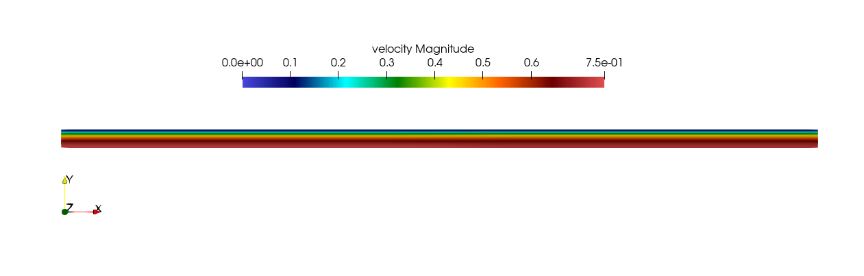
../_images/velocity_paraview.png — Fig. 5 Steady-State flow field visualized in Visit/ParaView. Colors represent velocity magnitude.

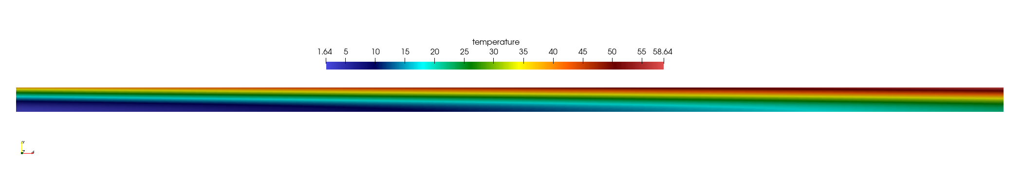
../_images/temp.png — Fig. 6 Temperature profile visualized in Visit/ParaView.

Plots of the velocity and temperature varying along the y-axis as evaluated by NekRS compared to the analytic solutions provided by Eqs. (1) and (2) respectively are shown below in Fig. 7 and Fig. 8.

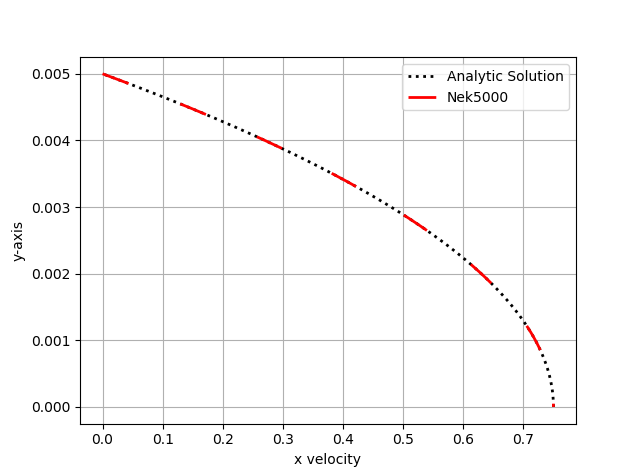
../_images/velocity_lineplot.png — Fig. 7 *Nek5000* velocity solutions plotted against analytical solutions.

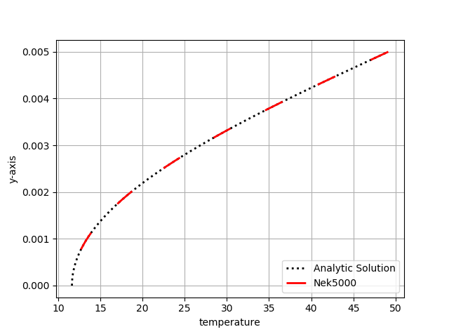
../_images/temperature_lineplot.png — Fig. 8 *Nek5000* temperature solutions plotted against analytical solutions.